16

Railway Track Maintenance

16.1 Introduction

Railway track is not a permanent structure in the traditional civil engineering sense: it degrades continuously under repeated traffic loading, environmental exposure, and the cumulative effects of countless wheel–rail interactions. Without systematic maintenance, track geometry deteriorates to the point where safe and comfortable train operation becomes impossible [124, 65].

Maintenance represents the largest recurring cost category in railway infrastructure management. On the Norwegian network (Bane NOR), the annual maintenance budget typically equals or exceeds the annual investment budget for renewal. The 2023–2024 Bane NOR infrastructure accounts indicate that the network comprises approximately 4200 km of track, of which significant proportions are over 20 or even 40 years old. Older track requires progressively more intensive maintenance to sustain the same level of service. Maintenance planning therefore has to cover not only rails, sleepers and ballast, but also the wider infrastructure asset classes shown in Figure 16.1.

Figure 16.1 Railway infrastructure components and asset classes relevant for maintenance planning.

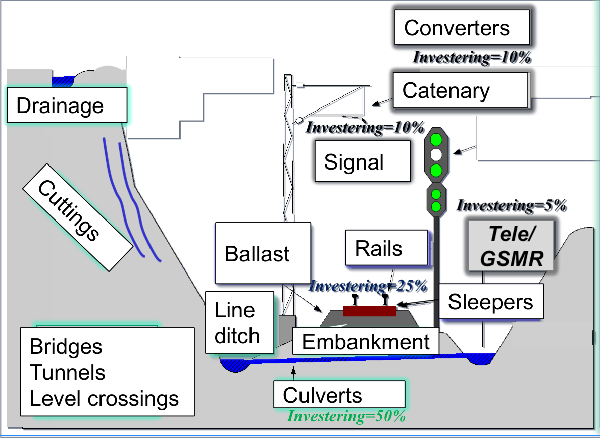
The primary goal of track maintenance is to preserve track geometry within the tolerance limits specified by Bane NOR technical regulations [10]. Secondary goals include extending component service life, preventing sudden failures, and ensuring cost-effective use of the maintenance budget. A structured approach that combines planned preventive activities with condition monitoring and corrective responses is essential to meet these goals while minimising traffic disruption.

16.2 Maintenance Types and Strategies

Maintenance strategy determines whether work is triggered by failure, fixed intervals, or measured condition. The distinction matters because each strategy gives a different balance between cost, traffic disruption, and risk.

16.2.1 Classification of Maintenance Types

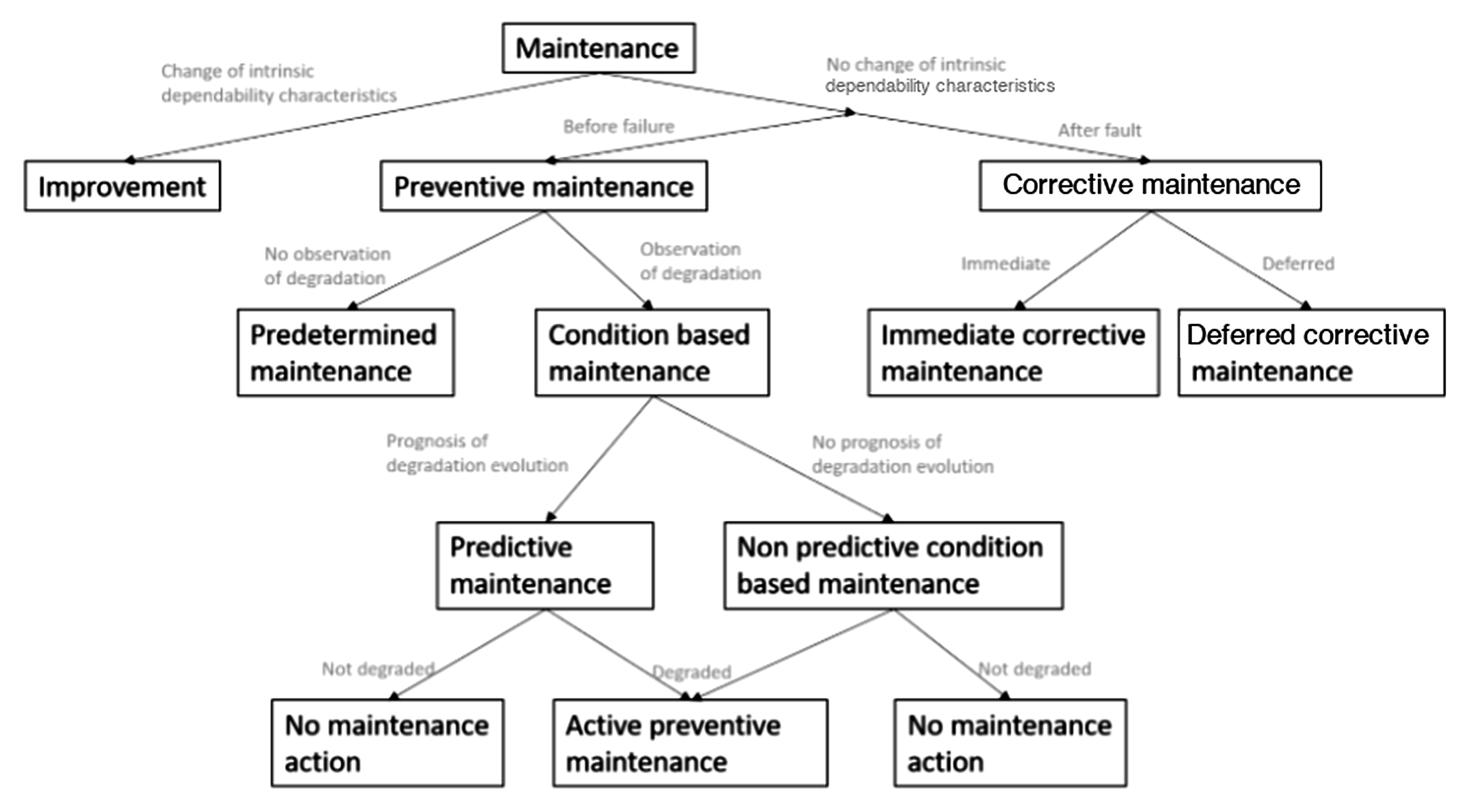
Railway maintenance is classified into three broad types based on when the intervention occurs relative to failure [124]:

Corrective maintenance (reactive maintenance) is carried out after a defect has been detected or a component has failed. It restores functionality but does not prevent recurrence. Examples include emergency rail replacement after a fracture, re-gauging after a misaligned fastening, or emergency re-levelling after a subgrade failure. Corrective maintenance is generally the most expensive type per unit of work because it often requires unplanned track possessions, premium labour rates, and urgent material procurement.

Preventive maintenance is carried out at predetermined intervals or when condition indicators reach defined thresholds, before failure occurs. The objective is to restore the track to a "like new" condition and reset the degradation process. The most important preventive maintenance operation for ballasted track is tamping, which corrects accumulated geometry errors by lifting sleepers and compacting ballast beneath them. Preventive grinding of rails removes surface rolling contact fatigue (RCF) cracks before they penetrate to the dangerous sub-surface zone.

Improvement maintenance (renewal or upgrading) goes beyond restoring the original condition: it replaces worn components with new or superior ones, or upgrades the track to a higher standard. Examples include replacing wooden sleepers with concrete sleepers, upgrading from UIC 54 to 60E1 rail, and installing continuous welded rail (CWR) on jointed sections.

The taxonomy in Figure 16.2 separates maintenance by the trigger for the work: a detected failure, a fixed interval, or a measured condition.

Figure 16.2 Maintenance strategy taxonomy.

Maintenance strategies differ by whether they prevent deterioration, restore condition after degradation, or renew components at the end of service life.

Strategy	Advantages	Limitations
Corrective	Low immediate planning cost.	High disruption, high safety exposure, and often expensive short-notice possessions.
Preventive	Predictable possessions and resource planning.	May replace or disturb assets before their full technical life is used.
Condition-based	Uses measured condition and degradation trends.	Requires reliable inspection data, thresholds, and trend interpretation.
Improvement	Provides long-term performance gain or capacity for higher loads/speeds.	Requires larger investment and possession demand.

Table 16.1 Advantages and limitations of common railway maintenance strategies.

In Norwegian corrective-maintenance planning, the response is also classified by urgency. Akutt korrektivt vedlikehold (AKV) is undertaken without delay to avoid unacceptable consequences. Utsatt korrektivt vedlikehold (UKV) is planned within a defined response category: UKV1 for a high probability of a safety-critical or service-stopping failure within 30 days, UKV2 for a high probability of a service-stopping failure within 365 days, and UKV3 where such a failure is not considered likely within those periods. The category must be based on consequence and deterioration risk, not merely on how visible the defect appears [44].

16.2.2 Worked Example: Maintenance Response Classification

Question. Classify the response to four observations from a weekly maintenance review. Assume that each observation has been confirmed and that the stated consequence assessment is valid.

Case	Observation	Classification and reason
A	A signal remains at red and prevents normal route operation.	AKV: restore the required function without delay and manage traffic until it is restored.
B	A culvert is partly blocked immediately before a period of forecast heavy rainfall.	UKV1: the near-term probability and consequence of rapid water-level rise justify action within 30 days, normally sooner.
C	Track-circuit values are approaching the service limit because the ballast is contaminated, but operation remains stable.	UKV2: plan corrective ballast/drainage work within the annual horizon before a service-stopping failure develops.
D	One isolated sleeper is defective, while gauge, fastening restraint, and neighbouring sleepers remain satisfactory.	UKV3: record and plan the replacement; the isolated condition does not currently indicate a likely stopping failure.

Decision flow. First identify the lost or threatened function. Then estimate the time horizon to a safety-critical or service-stopping consequence. Finally, choose the response category and document any temporary controls, inspection interval, possession, materials, and completion deadline. The same physical defect may move from UKV3 to UKV1 if its extent, traffic exposure, weather, or degradation rate changes. A defensible decision combines this urgency logic with measured geometry and condition trends rather than classifying from appearance alone.

16.2.3 The Bathtub Curve and Degradation Modelling

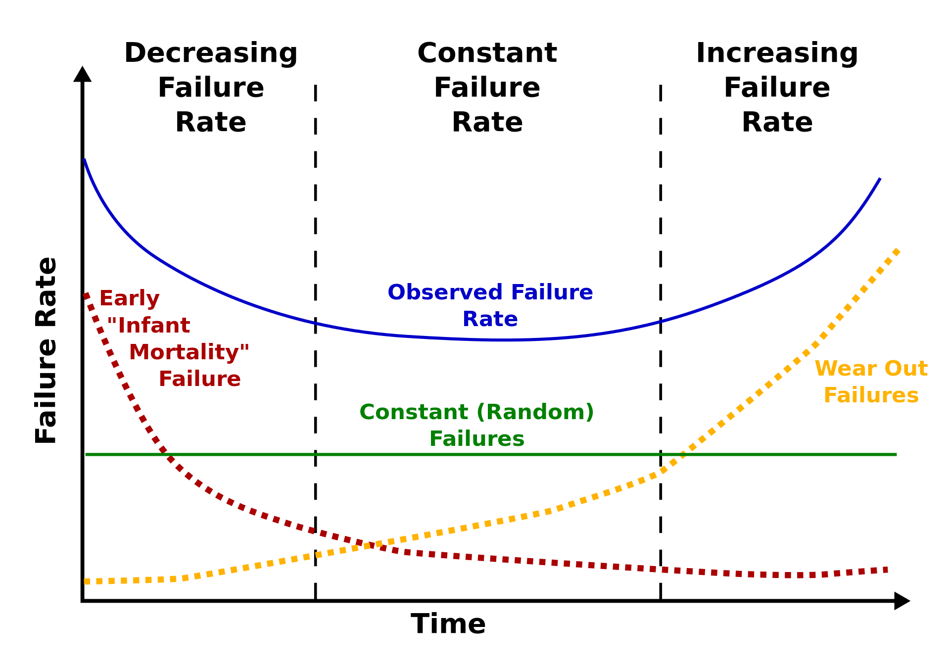
The service life of a track component can be described by the bathtub curve, which plots the instantaneous failure rate against time [124]:

• Early or "infant mortality" failures: The left-hand part of Figure 16.3 shows a decreasing failure rate. Failures are initially more likely because new or recently disturbed components are still bedding in, installation defects may be exposed, and ballast disturbed by tamping or renewal is consolidating under traffic.

• Constant or random failures: The middle part of the curve represents a roughly constant failure rate. For track assets this is the target operating regime, where failures are not mainly caused by age but by random events, local defects, unusual loads, drainage problems, or isolated component weaknesses.

• Wear-out failures: The right-hand part of the curve shows an increasing failure rate as fatigue damage, wear, corrosion, ballast fouling, and material degradation accumulate. In this region corrective maintenance becomes less effective, and renewal or major intervention becomes economically necessary.

The blue observed failure-rate curve in Figure 16.3 is the combined effect of these three mechanisms. It explains why newly disturbed track, mature track and worn-out components require different inspection and maintenance responses.

Figure 16.3 Bathtub curve showing early failures, constant random failures and wear-out failures over service time.

16.2.4 Norwegian Maintenance Strategy

Bane NOR's maintenance strategy is based on the principle of condition-based preventive maintenance: inspections and measurements are carried out at regular intervals, and maintenance work is triggered when condition indicators fall below defined thresholds, rather than at fixed calendar intervals [10, 145].

Key elements of the Norwegian strategy include:

• Track geometry measurement by the diagnostic train (målevogn) typically 2–4 times per year on main lines.

• Automated analysis of geometry data to calculate quality indices (TQI) and identify sections requiring intervention.

• Risk-based prioritisation: sections with high traffic, high speed, or safety-critical geometry errors receive priority intervention.

• Life-cycle planning: renewal decisions are based on whole-life cost analysis comparing continued maintenance with component replacement.

16.3 Track Geometry Quality

Track geometry quality is the part of maintenance most directly tied to what is measured on the track. The purpose is not only to name the geometry parameters, but to see what they look like, understand how they are measured, and then read the tolerance limits that decide whether the defect can wait for planned maintenance or needs immediate attention. The presentation below follows the same sequence for each parameter: definition, figure, tolerance table, and maintenance interpretation.

Diagnostic trains measure the geometry continuously at line speed, while local follow-up can use manual gauges, chord measurements and levelling. Figure 16.4 gives the compact overview: gauge acts across the rails, longitudinal level acts vertically along each rail, horizontal alignment acts laterally in plan, cross-level or cant acts between the rails, and twist is the change in cant over a measuring base.

Figure 16.4 Track geometry quantities used for maintenance assessment: gauge, level, alignment, cant and twist [89, 48].

16.3.1 Quality Classes and Limit Levels

Bane NOR technical regulations classify geometry limits by quality class, measurement basis and wavelength band [44, 48]. The quality class follows the highest permitted line speed, as shown in Table 16.2.

Quality class	Line speed
Q0	\(230 < V \leq 300\) km/h
Q1	\(160 < V \leq 230\) km/h
Q2	\(120 < V \leq 160\) km/h
Q3	\(80 < V \leq 120\) km/h
Q4	\(40 < V \leq 80\) km/h
Q5	\(V \leq 40\) km/h

Table 16.2 Bane NOR quality classes for track-geometry maintenance limits [44].

Worked examples may use an individual quality class, such as Q2, but the regulation covers all quality classes rather than a single row. The full Bane NOR rows are therefore reproduced below for each parameter. The limit levels should be read as follows: exceeding the maintenance limit means the defect should enter the planned maintenance programme; exceeding the action limit means the defect must be corrected and followed up before it can develop into an immediate defect; and exceeding the immediate limit means prompt repair and, where required, speed reduction until the defect is removed. Values in the following tables are in millimetres unless stated otherwise.

16.3.2 Track Gauge

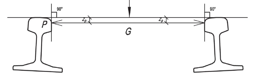
Track gauge is the distance between the inner rail faces. In the standard definition used for maintenance, it is measured at the gauge point below the running surface, not across the top of the rail head. In Figure 16.5, \(l_p\) denotes this vertical gauge-point depth; the standard track gauge \(G\) is measured between the inner running edges \(14\) mm below the rail-head top [48]. On the Norwegian network the nominal gauge is 1435 mm, so a gauge defect is read as a deviation from 1435 mm.

Figure 16.5 Track gauge G measured at l_p = 14 mm below the rail-head top.

Class	Line speed	New track	Maintenance	Action	Immediate
Q0	\(230 < V \leq 300\) km/h	+3/-0	+10/-3	+15/-4	+28/-5
Q1	\(160 < V \leq 230\) km/h	+4/-0	+12/-4	+20/-5	+28/-7
Q2	\(120 < V \leq 160\) km/h	+4/-0	+15/-5	+25/-6	+35/-8
Q3	\(80 < V \leq 120\) km/h	+4/-3	+15/-7	+30/-8	+35/-9
Q4	\(40 < V \leq 80\) km/h	+4/-4	+20/-7	+30/-8	+35/-9
Q5	\(V \leq 40\) km/h	+5/-5	+20/-7	+30/-8	+35/-9

Table 16.3 Bane NOR limits for deviation in track gauge from the nominal 1435 mm gauge [48].

Class	Line speed	Maintenance	Action
Q0	\(230 < V \leq 300\) km/h	7	10
Q1	\(160 < V \leq 230\) km/h	8	10
Q2	\(120 < V \leq 160\) km/h	9	10
Q3	\(80 < V \leq 120\) km/h	10	15
Q4	\(40 < V \leq 80\) km/h	12	18
Q5	\(V \leq 40\) km/h	15	25

Table 16.4 Bane NOR limits for change in track gauge over 10 m track length [48].

The first table controls how far the gauge may be from nominal. The second table controls how quickly it changes along the track, because a sudden change can be more critical for vehicle guidance than a slowly varying offset. Gauge widening is commonly linked to rail wear, rail head deformation, rail roll, loose fastenings, sleeper deterioration or poor construction control. Typical maintenance actions are correcting rail position, replacing fastenings or sleepers, and replacing worn rail where the gauge can no longer be held.

16.3.3 Longitudinal Level

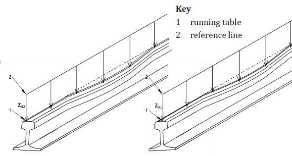
Longitudinal level is the vertical position of each rail along the track. Figure 16.6 shows the measured running table compared with a smoothed reference line. The quantity is therefore not the absolute elevation of the track; it is the vertical deviation from the reference line within a specified wavelength band. Bane NOR gives separate limit tables for D1 (3–25 m) and D2 (25–70 m).

Figure 16.6 Longitudinal level as vertical deviation from a reference line.

Class	Line speed	New	Newly adjusted	Maintenance	Action	Immediate
Q0	\(230 < V \leq 300\) km/h	\(\pm 2\)	\(\pm 2\)	\(\pm 6\)	\(\pm 8\)	\(\pm 16\)
Q1	\(160 < V \leq 230\) km/h	\(\pm 2\)	\(\pm 2\)	\(\pm 6\)	\(\pm 9\)	\(\pm 20\)
Q2	\(120 < V \leq 160\) km/h	\(\pm 2\)	\(\pm 2\)	\(\pm 10\)	\(\pm 12\)	\(\pm 23\)
Q3	\(80 < V \leq 120\) km/h	\(\pm 3\)	\(\pm 4\)	\(\pm 13\)	\(\pm 16\)	\(\pm 26\)
Q4	\(40 < V \leq 80\) km/h	\(\pm 3\)	\(\pm 5\)	\(\pm 15\)	\(\pm 19\)	\(\pm 28\)
Q5	\(V \leq 40\) km/h	\(\pm 3\)	\(\pm 6\)	\(\pm 17\)	\(\pm 21\)	\(\pm 28\)

Table 16.5 Bane NOR limits for longitudinal level irregularity in wavelength band D1 (3–25 m) [48].

Class	Line speed	New	Newly adjusted	Maintenance	Action	Immediate
Q0	\(230 < V \leq 300\) km/h	\(\pm 7\)	\(\pm 7\)	\(\pm 10\)	\(\pm 14\)	\(\pm 18\)
Q1	\(160 < V \leq 230\) km/h	\(\pm 7\)	\(\pm 7\)	\(\pm 12\)	\(\pm 16\)	\(\pm 24\)
Q2	\(120 < V \leq 160\) km/h	–	–	–	–	–
Q3	\(80 < V \leq 120\) km/h	–	–	–	–	–
Q4	\(40 < V \leq 80\) km/h	–	–	–	–	–
Q5	\(V \leq 40\) km/h	–	–	–	–	–

Table 16.6 Bane NOR limits for longitudinal level irregularity in wavelength band D2 (25–70 m) [48].

Longitudinal-level defects increase dynamic wheel loads and often reveal differential settlement, unstable support, frost heave, ballast pockets or incorrect tamping. If the vertical defect is mainly on one rail, the same support problem may also create twist. The usual remedy is tamping; if the defect returns quickly, the drainage, ballast or subgrade condition should be corrected before repeated tamping is specified.

16.3.4 Horizontal Alignment

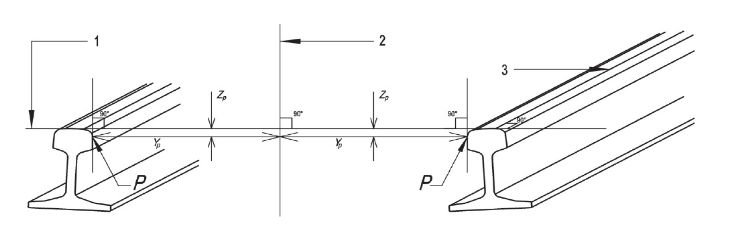
Horizontal alignment is the lateral position of the rails in plan. Figure 16.7 shows the side error relative to a horizontal reference line. In maintenance, this is commonly evaluated as a versine or lateral deviation within the wavelength band, so the limit is much tighter than a visual estimate of the track centreline would suggest.

Figure 16.7 Horizontal alignment as lateral deviation from a reference line.

Class	Line speed	New	Newly adjusted	Maintenance	Action	Immediate
Q0	\(230 < V \leq 300\) km/h	\(\pm 2\)	\(\pm 2\)	\(\pm 3\)	\(\pm 4\)	\(\pm 10\)
Q1	\(160 < V \leq 230\) km/h	\(\pm 2\)	\(\pm 2\)	\(\pm 3\)	\(\pm 4\)	\(\pm 12\)
Q2	\(120 < V \leq 160\) km/h	\(\pm 2\)	\(\pm 2\)	\(\pm 4\)	\(\pm 5\)	\(\pm 14\)
Q3	\(80 < V \leq 120\) km/h	\(\pm 2\)	\(\pm 3\)	\(\pm 5\)	\(\pm 7\)	\(\pm 17\)
Q4	\(40 < V \leq 80\) km/h	\(\pm 2\)	\(\pm 3\)	\(\pm 8\)	\(\pm 11\)	\(\pm 22\)
Q5	\(V \leq 40\) km/h	\(\pm 2\)	\(\pm 4\)	\(\pm 10\)	\(\pm 14\)	\(\pm 22\)

Table 16.7 Bane NOR limits for horizontal alignment irregularity in wavelength band D1 (3–25 m) [48].

Class	Line speed	New	Newly adjusted	Maintenance	Action	Immediate
Q0	\(230 < V \leq 300\) km/h	\(\pm 5\)	\(\pm 5\)	\(\pm 10\)	\(\pm 12\)	\(\pm 14\)
Q1	\(160 < V \leq 230\) km/h	\(\pm 5\)	\(\pm 5\)	\(\pm 11\)	\(\pm 16\)	\(\pm 18\)
Q2	\(120 < V \leq 160\) km/h	–	–	–	–	–
Q3	\(80 < V \leq 120\) km/h	–	–	–	–	–
Q4	\(40 < V \leq 80\) km/h	–	–	–	–	–
Q5	\(V \leq 40\) km/h	–	–	–	–	–

Table 16.8 Bane NOR limits for horizontal alignment irregularity in wavelength band D2 (25–70 m) [48].

Alignment defects may come from lining or tamping with poor input data, abrupt cant transitions, insufficient lateral ballast resistance, poor ballast shoulder condition or high internal rail forces. Poor alignment reduces ride comfort, increases lateral forces in fastenings and ballast, and accelerates uneven rail wear. The normal maintenance response is lining combined with tamping and ballast consolidation.

16.3.5 Cross-Level

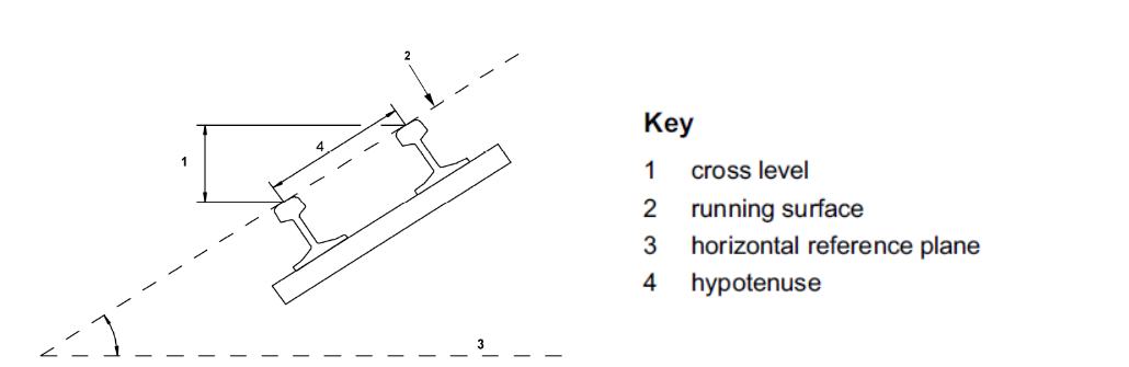
Cross-level is the height difference between the two rails at a cross-section. In maintenance data, the cross-level irregularity is the local deviation from the intended or mean cant value. Figure 16.8 shows the cross-section definition used in EN track-geometry terminology [89]. Local peaks and dips relative to the intended cant profile are the irregularities that enter the tolerance check.

Figure 16.8 Cross-level/cant definition: the height difference between the two running rails.

Class	Line speed	Newly adjusted	Maintenance	Action
Q0	\(230 < V \leq 300\) km/h	\(\pm 3\)	\(\pm 6\)	\(\pm 8\)
Q1	\(160 < V \leq 230\) km/h	\(\pm 3\)	\(\pm 6\)	\(\pm 8\)
Q2	\(120 < V \leq 160\) km/h	\(\pm 4\)	\(\pm 6\)	\(\pm 9\)
Q3	\(80 < V \leq 120\) km/h	\(\pm 4\)	\(\pm 8\)	\(\pm 11\)
Q4	\(40 < V \leq 80\) km/h	\(\pm 5\)	\(\pm 10\)	\(\pm 13\)
Q5	\(V \leq 40\) km/h	\(\pm 5\)	\(\pm 10\)	\(\pm 15\)

Table 16.9 Bane NOR limits for cross-level irregularity, measured as deviation from the 20 m mean cant [48].

Cross-level defects are commonly caused by poor construction quality, differential settlement, ballast voids, subgrade movement or an incorrect initial cant. They can be measured manually with a track gauge and level, or continuously by a measuring train. The usual remedy is tamping with controlled lifting of the low or high rail according to the design geometry.

16.3.6 Cant

Cant is the same physical height difference between rails, but read as the intended superelevation on a curve. Figure 16.8 shows the cross-section definition: the rail running surface is compared with a horizontal reference plane, and the vertical leg is reported as cant or cross-level. For curved track, the absolute cant is controlled in addition to local cross-level irregularity.

Line type	Action	Immediate
Mixed-traffic line	\(>150\)	180
Passenger line	\(>180\)	190

Table 16.10 Bane NOR tolerance limits for absolute cant by line type [48].

Too much cant can overload the low rail or give poor behaviour for slow and freight trains; too little cant or high cant deficiency increases lateral wheel–rail forces. The maintenance decision is therefore not only whether the local track is uneven, but whether the curve geometry still matches the intended traffic speed and traffic mix.

16.3.7 Track Twist

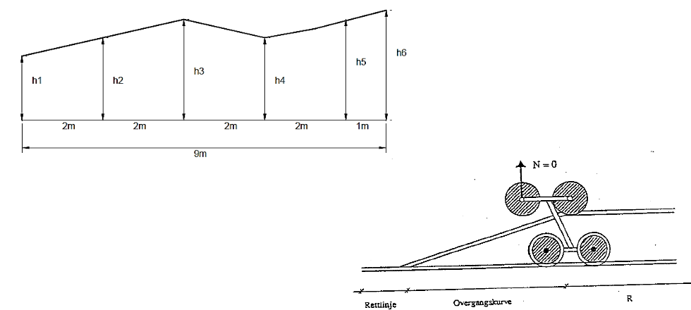
Track twist is the change in cross-level over a specified measuring base. Figure 16.9 shows why this is different from absolute cant: a track can have acceptable cant at each point but still change too rapidly between points. Bane NOR uses both 2 m and 9 m bases in the tolerance checks.

Figure 16.9 Track twist as a change in cross-level over a measuring base.

Class	Line speed	New	Newly adjusted	Maint.	Action	Imm. \(R \geq 400\)	Imm. \(R < 400\)
Q0	\(230 < V \leq 300\) km/h	\(\pm 2\)	\(\pm 2\)	\(\pm 6\)	\(\pm 7\)	\(\pm 10\)	–
Q1	\(160 < V \leq 230\) km/h	\(\pm 2\)	\(\pm 2\)	\(\pm 6\)	\(\pm 7\)	\(\pm 10\)	–
Q2	\(120 < V \leq 160\) km/h	\(\pm 2\)	\(\pm 2\)	\(\pm 7\)	\(\pm 10\)	\(\pm 14\)	–
Q3	\(80 < V \leq 120\) km/h	\(\pm 3\)	\(\pm 3\)	\(\pm 7\)	\(\pm 10\)	\(\pm 14\)	\(\pm 12\)
Q4	\(40 < V \leq 80\) km/h	\(\pm 4\)	\(\pm 4\)	\(\pm 7\)	\(\pm 10\)	\(\pm 14\)	\(\pm 12\)
Q5	\(V \leq 40\) km/h	\(\pm 5\)	\(\pm 5\)	\(\pm 7\)	\(\pm 10\)	\(\pm 14\)	\(\pm 12\)

Table 16.11 Bane NOR limits for track twist with 2 m measuring base [48].

Class	Line speed	New	Newly adjusted	Maint.	Action	Imm. \(R \geq 400\)	Imm. \(R < 400\)
Q0	\(230 < V \leq 300\) km/h	\(\pm 6\)	\(\pm 6\)	\(\pm 24\)	\(\pm 31\)	\(\pm 43\)	–
Q1	\(160 < V \leq 230\) km/h	\(\pm 6\)	\(\pm 6\)	\(\pm 24\)	\(\pm 31\)	\(\pm 43\)	–
Q2	\(120 < V \leq 160\) km/h	\(\pm 6\)	\(\pm 6\)	\(\pm 24\)	\(\pm 31\)	\(\pm 43\)	–
Q3	\(80 < V \leq 120\) km/h	\(\pm 6\)	\(\pm 6\)	\(\pm 24\)	\(\pm 31\)	\(\pm 43\)	\(\pm 34\)
Q4	\(40 < V \leq 80\) km/h	\(\pm 9\)	\(\pm 9\)	\(\pm 24\)	\(\pm 31\)	\(\pm 43\)	\(\pm 34\)
Q5	\(V \leq 40\) km/h	\(\pm 15\)	\(\pm 15\)	\(\pm 24\)	\(\pm 31\)	\(\pm 43\)	\(\pm 34\)

Table 16.12 Bane NOR limits for track twist with 9 m measuring base [48].

Twist is safety-critical because it can unload one wheel, especially for torsionally stiff vehicles. It may be caused by local settlement, frost heave, isolated ballast pockets, construction work or an abrupt cant ramp in transition geometry. Measuring trains detect twist continuously, while local checks can be made manually over the prescribed bases. The maintenance response is usually tamping or manual packing to restore the cross-level sequence; if excess ballast has created a local high point, ballast removal may be needed before the track is handed back.

16.3.8 Track Quality Index (TQI), K-Number and Position Checks

Instead of evaluating individual defects in isolation, infrastructure managers also use section-based quality indicators. In the international literature, Track Quality Index (TQI) is not one universal formula: most versions combine statistical features of measured track-geometry signals, especially standard deviations over a defined section length. Bane NOR's operational quality measure is the quality number, K-tallet, which expresses how large a share of the section has all standard-deviation values within the quality limits [16, 96, 48].

For one geometry parameter \(x\), measured at \(n\) points in a calculation window, the mean and standard deviation are

\[ \bar{x}=\frac{1}{n}\sum_{i=1}^{n}x_i, \qquad \sigma_x=\sqrt{\frac{1}{n}\sum_{i=1}^{n}(x_i-\bar{x})^2}. \]

Here \(x_i\) is a measured deviation in millimetres, for example longitudinal level or horizontal alignment. Under the Bane NOR assessment method, these standard deviations are normally calculated over 200 m or 1000 m sections; assessment diagrams use a moving 200 m basis and report K- and Q-values for each full kilometre [16].

Bane NOR's quality table uses the following standard-deviation checks:

\[ \begin{aligned} \sigma_H &= \sigma(\text{vertical geometry}), & \sigma_R &= \sigma(\text{cant}),\\ \sigma_P &= \sigma(\text{horizontal geometry}), & \sigma_S &= \sqrt{\sigma_R^2+\sigma_P^2}. \end{aligned} \]

The interaction value \(\sigma_S\) is therefore a vector sum used when combined cant and horizontal irregularity is more critical than either parameter alone. Generic TQI methods often combine several standard deviations as a weighted sum or a combined standard deviation,

\[ \mathrm{TQI}_{\mathrm{SD}}=\sum_{j=1}^{m} w_j\sigma_j, \qquad \mathrm{CoSD}=\sqrt{\sum_{j=1}^{m} w_j\sigma_j^2}, \]

where the weights \(w_j\), parameters, and aggregation length are railway-specific. These generic forms are useful for comparing concepts, but the maintenance decision in this chapter should use the Bane NOR K-number and quality limits in Tables 16.13 and 16.14.

For a section of length \(L\), the K-number is calculated as

\[ K=100\,\frac{\sum l_{\mathrm{OK}}}{L}, \]

where \(\sum l_{\mathrm{OK}}\) is the total length where all relevant \(\sigma\)-values are within the quality limits.

Class	Line speed	\(\boldsymbol{\sigma_H}\) vertical	\(\boldsymbol{\sigma_R}\) cant	\(\boldsymbol{\sigma_P}\) horizontal	\(\boldsymbol{\sigma_S}\) interaction
Q0	\(230 < V \leq 300\) km/h	0.85	0.90	0.50	1.60
Q1	\(160 < V \leq 230\) km/h	1.15	1.00	0.70	1.70
Q2	\(120 < V \leq 160\) km/h	1.40	1.20	0.75	1.90
Q3	\(80 < V \leq 120\) km/h	1.80	1.40	1.05	2.40
Q4	\(40 < V \leq 80\) km/h	2.75	1.80	1.95	3.10
Q5	\(V \leq 40\) km/h	2.75	2.20	1.95	3.60

Table 16.13 Bane NOR standard-deviation quality limits used for K-number calculation; all $\sigma$-values are in millimetres [16, 48].

Class	Line speed	Newly adjusted	Maintenance	Action
Q0	\(230 < V \leq 300\) km/h	90	90	80
Q1	\(160 < V \leq 230\) km/h	90	90	75
Q2	\(120 < V \leq 160\) km/h	90	90	50
Q3	\(80 < V \leq 120\) km/h	90	80	30
Q4	\(40 < V \leq 80\) km/h	90	75	20
Q5	\(V \leq 40\) km/h	–	–	–

Table 16.14 Bane NOR requirements for the quality number $K$ [48].

16.3.8.1 Worked Example: TQI and K-Number

Consider a 1000 m Q2 section divided into five 200 m assessment windows: 0–200, 200–400, 400–600, 600–800 and 800–1000 m. Table 16.15 gives the input values from the measuring train. The detailed calculation below is for the 400–600 m window only; it is a 200 m window located between chainage 400 m and 600 m.

Assessment window	\(\boldsymbol{\sigma_H}\)	\(\boldsymbol{\sigma_R}\)	\(\boldsymbol{\sigma_P}\)
0–200 m	1.10	0.80	0.50
200–400 m	1.35	1.05	0.70
400–600 m	1.70	1.40	0.90
600–800 m	1.20	1.10	0.72
800–1000 m	1.30	0.90	0.60

Table 16.15 Input values for the Q2 TQI and K-number example; all $\sigma$-values are in millimetres.

The interaction value for each window is calculated as

\[ \sigma_S=\sqrt{\sigma_R^2+\sigma_P^2}. \]

For the 400–600 m window in Table 16.15,

\[ \sigma_S=\sqrt{1.40^2+0.90^2}=1.66~\mathrm{mm}. \]

To illustrate how a generic TQI can be calculated from the same values, use the Q2 limits in Table 16.13 as denominators in an equal-weight, normalised comparison index:

\[ \mathrm{TQI}_{\mathrm{norm}}= \frac{1}{4}\left( \frac{\sigma_H}{1.40} +\frac{\sigma_R}{1.20} +\frac{\sigma_P}{0.75} +\frac{\sigma_S}{1.90} \right), \]

For the 400–600 m window this gives

\[ \mathrm{TQI}_{\mathrm{norm}}= \frac{1}{4}\left( \frac{1.70}{1.40} +\frac{1.40}{1.20} +\frac{0.90}{0.75} +\frac{1.66}{1.90} \right)=1.11. \]

This normalised TQI is useful for ranking roughness, but the Bane NOR K-number decision is stricter: a 200 m window is counted as OK only when all four standard-deviation checks satisfy the Q2 limits.

Window	\(\boldsymbol{\sigma_H}\)	\(\boldsymbol{\sigma_R}\)	\(\boldsymbol{\sigma_P}\)	\(\boldsymbol{\sigma_S}\)	\(\boldsymbol{\mathrm{TQI}_{\mathrm{norm}}}\)	OK length
0–200 m	1.10	0.80	0.50	0.94	0.65	200 m
200–400 m	1.35	1.05	0.70	1.26	0.86	200 m
400–600 m	1.70	1.40	0.90	1.66	1.11	0 m
600–800 m	1.20	1.10	0.72	1.31	0.86	200 m
800–1000 m	1.30	0.90	0.60	1.08	0.76	200 m

Table 16.16 Worked Q2 example for TQI ranking and K-number calculation; all $\sigma$-values are in millimetres and $\mathrm{TQI}_{\mathrm{norm}}$ is dimensionless.

The 400–600 m window is not OK because \(\sigma_H=1.70>1.40\), \(\sigma_R=1.40>1.20\), and \(\sigma_P=0.90>0.75\), even though the interaction value \(\sigma_S=1.66\) remains below 1.90. The OK length is therefore

\[ \sum l_{\mathrm{OK}}=200+200+0+200+200=800~\mathrm{m}. \]

The K-number for the 1000 m section is

\[ K=100\,\frac{800}{1000}=80. \]

For a Q2 line this is below the maintenance limit of 90, but above the action limit of 50. The section should therefore enter root-cause investigation and planned tamping or renewal assessment before the quality drops into the action range. In this example, the failed window also has the highest normalised TQI, so it is the first 200 m part of the kilometre to inspect in the field.

Class	Line speed	Newly adjusted	Maintenance
Q0–Q1	\(160 < V \leq 300\) km/h	+10/-20	+20/-30
Q2–Q5	\(V \leq 160\) km/h	+30/-40	+50/-75

Table 16.17 Bane NOR limits for absolute vertical track position when fixed reference points are used [48].

Class	Line speed	Curve radius	Newly adjusted	Maintenance
Q0–Q1	\(160 < V \leq 300\) km/h	–	\(\pm 20\)	\(\pm 30\)
Q2–Q5	\(V \leq 160\) km/h	\(R>1000\) m	\(\pm 40\)	\(\pm 60\)
Q2–Q5	\(V \leq 160\) km/h	\(750<R\leq1000\) m	\(\pm 40\)	\(\pm 40\)
Q2–Q5	\(V \leq 160\) km/h	\(500<R\leq750\) m	\(\pm 30\)	\(\pm 30\)
Q2–Q5	\(V \leq 160\) km/h	\(350<R\leq500\) m	\(\pm 20\)	\(\pm 20\)
Q2–Q5	\(V \leq 160\) km/h	\(R\leq350\) m	\(\pm 15\)	\(\pm 15\)

Table 16.18 Bane NOR limits for absolute horizontal track position [48].

16.4 Track Inspection

Track inspection is the input side of maintenance planning. It converts observations and measurements into decisions: continue monitoring, plan tamping or grinding, repair a component, impose a restriction, or prepare a renewal. Chapter 17, Section 17.2, describes the measuring vehicles and sensor systems; the defect types feeding the inspection process are described in Chapter 15. This section focuses on how inspection results are used by the maintenance engineer.

Walking inspection (linjevisitasjon) is used to find visible defects and local conditions that are difficult to judge from a measurement trace alone: broken sleepers, missing or loose fastenings, ballast shoulder loss, blocked drainage, vegetation, mud pumping, rail-surface damage and poor local access conditions.

Figure 16.10 Turnout field measurement showing the track component, measuring equipment and digital recording in one inspection setting.

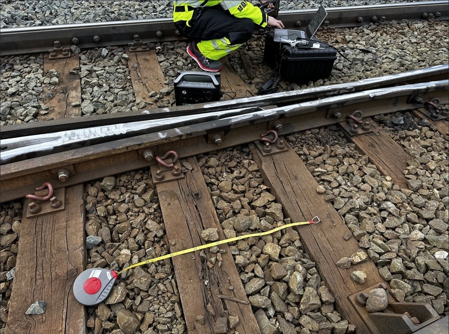
Rail-flaw testing checks whether the rail contains internal or surface-breaking defects that require repair, closer monitoring or rail replacement. The maintenance decision is based on defect type, defect size, rail stress state, traffic load and the time available before the next safe work possession.

Diagnostic geometry measurement provides the measured parameters used in Section 16.3: gauge, longitudinal level, horizontal alignment, cross-level/cant and twist. The outputs are compared with the alert, intervention and immediate-action limits in the technical regulations. A diagnostic train such as ROGER 1000 therefore belongs in Chapter 17 as a measuring vehicle; in this chapter it matters as the source of the maintenance work list.

Inspection frequency is line-class and risk dependent. The practical principle is that high-speed, high-tonnage and safety-critical sections are inspected more often than lightly trafficked secondary lines. The maintenance engineer then combines the latest inspection results with degradation trend, traffic consequence and possession availability before choosing the intervention.

16.5 Tamping

Tamping is the normal maintenance response when poor vertical level, alignment or cross-level is still caused mainly by sleeper support and ballast packing rather than by life-expired components. Tamping machines lift and line the track and pack ballast under the sleepers; the machinery and tamping sequence are described in Chapter 17, Section 17.4, especially Figure 17.9. In this chapter the maintenance question is when tamping is the right intervention.

Tamping is suitable when the geometry defect is moderate, the ballast can still provide stable support after re-packing, and the corrected geometry will remain within limits until the next inspection. It is less suitable when the same location deteriorates rapidly after each pass. In that case the root cause may be fouled ballast, poor drainage, weak formation, rail-seat deterioration, sleeper damage or an unresolved transition-zone problem.

After tamping, the disturbed ballast is initially less stable than undisturbed ballast, and a short settlement period follows before re-consolidation. Traffic loading, dynamic track stabilisation and shoulder compaction can help restore stability after track work; where the required conditions are not yet documented, temporary speed restrictions may be needed [6].

Each tamping pass also crushes some ballast particles. Repeated tamping therefore has a maintenance cost beyond the possession itself: it shortens the remaining ballast life. When geometry correction no longer lasts, tamping should be replaced by drainage repair, ballast cleaning, ballast renewal or a more extensive track renewal decision.

16.6 Rail Grinding

Rail grinding removes material from the rail head to achieve two goals [65, 124]:

Preventive grinding removes the shallow surface layer (typically 0.1–0.3 mm) in which rolling contact fatigue (RCF) cracks initiate, before they penetrate to the dangerous depth (typically 3–5 mm). By removing this layer at regular intervals, rail service life can be extended substantially compared with a purely corrective strategy.

Corrective grinding removes existing cracks and restores the rail head profile. It requires deeper material removal (0.3–1.0 mm or more) and must be completed before cracks reach a depth requiring rail replacement.

Figure 16.11 shows the practical result of grinding in measured rail-corrugation output: the rougher trace before treatment is replaced by a much smoother trace after treatment. The grinding and milling machines themselves are described in Chapter 17, Section 17.3; here the important point is the maintenance strategy and timing of the intervention.

Figure 16.11 Measured rail-corrugation condition before and after rail grinding.

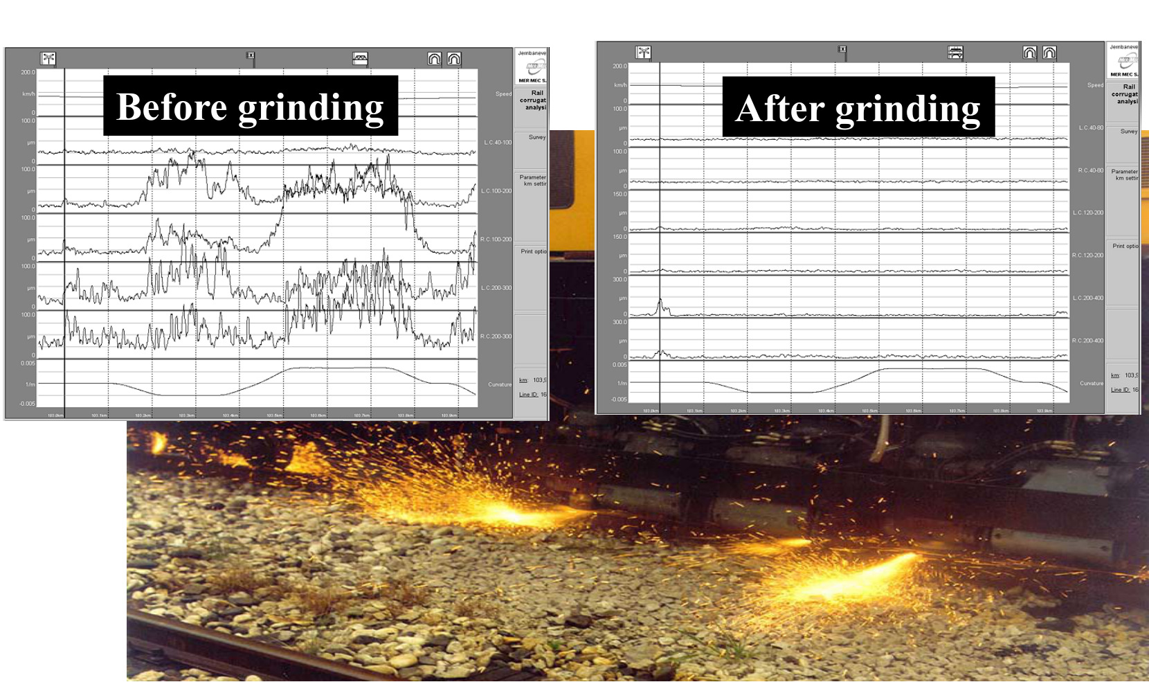
Grinding must be planned together with rail-profile measurements, rail-flaw information, noise or corrugation complaints, curve radius and traffic load. A preventive programme normally removes little metal per visit but repeats the work before cracks become deep. A corrective programme removes more metal, takes longer and consumes more of the rail head. The maintenance decision is therefore a balance between present defect removal and future rail life.

16.7 Ballast Cleaning and Renewal

As described in Chapter 3, ballast progressively fouls from particle breakdown, sleeper wear, and subgrade pumping. When fines content exceeds approximately 15–30% by mass, drainage and load-distribution functions are impaired.

Preventive ballast care aims to delay both crushing and contamination. Practical measures include using durable crushed rock, providing sufficient ballast depth below the sleeper, using under-sleeper pads where support is very stiff, keeping drainage open, avoiding unnecessary repeated tamping, preventing ore or freight leakage onto the track, controlling vegetation that drops organic material into the ballast, and ensuring that maintenance work does not introduce soil or fines into the ballast bed.

Ballast cleaning (ballastrensing) is selected when the coarse ballast can still be reused, but fines have reduced drainage and support. The maintenance objective is to remove the fouled fraction, restore drainage, add fresh ballast where needed, tamp the track and return the section to stable geometry. The ballast-cleaning machines and the excavation/screening workflow are described in Chapter 17, Section 17.5.

Full ballast replacement (ballastsanering) is selected when cleaning is no longer economical or technically sufficient. Typical triggers are heavily rounded or crushed ballast, recurring mud pumping, poor formation condition, repeated loss of geometry after tamping, or a renewal possession where sleepers and rails are replaced at the same time. Renewal trains and sleeper replacement systems are treated as machinery in Chapter 17, Section 17.6; in this chapter they are part of the maintenance decision about when local repair should become renewal.

16.8 Maintenance Cycles

Table 16.19 gives indicative maintenance and renewal cycles from railway maintenance literature for an intensively operated main line. The values are useful as order-of-magnitude planning figures for a Norwegian mixed-traffic main line carrying about 20–25 MGT/year, but they should not be read as Bane NOR limit values. Grinding is the most frequent intervention (every 1–3 years); subsoil rehabilitation is the least frequent (typically longer than 40 years).

Maintenance type	Passage [MGT]	Typical duration [years]
Tamping	40–70	4–5
Grinding	20–30	1–3
Ballast cleaning	150–300	12–15
Rail replacement	300–1000	10–15
Wooden sleeper replacement	250–600	20–30
Concrete sleeper replacement	350–700	30–40
Rail fastenings	100–500	10–30
Ballast replacement	200–500	20–30
Subsoil rehabilitation	\(>500\)	\(>40\)

Table 16.19 Typical maintenance intervention cycles for main track components on an intensively operated main line, adapted from Tzanakakis [154].

Whole-life cost analysis (LCC, Life Cycle Cost) provides the framework for comparing maintenance strategies. For a given track section, the LCC model calculates the net present value of all future maintenance and renewal costs under different intervention strategies. The strategy with the lowest LCC, subject to safety and service constraints, is selected.

16.9 CWR Stress Management and De-stressing

Continuously welded rail (CWR) is detailed in Chapter 9; from a maintenance perspective, the key challenge is ensuring that the neutral temperature \(T_n\) (the temperature at which the rail has zero longitudinal stress) remains close to the prescribed laying temperature throughout the rail's service life. Bane NOR technical regulations specify \(T_n=(21\pm3)\,^\circ\mathrm{C}\) for Norwegian main lines [11].

16.9.1 Causes of Neutral Temperature Shift

The neutral temperature of a CWR section can shift away from the original laying temperature as a result of:

Tamping: Each tamping pass disturbs the ballast and sleeper support and may laterally reposition the sleepers. If the rail is in a longitudinal stress state at the time of tamping, the ballast consolidation process re-anchors the track at a slightly different position, effectively shifting the neutral temperature. Repeated tamping without re-stressing can cause the neutral temperature to drift upward (increasing the risk of rail pull-apart in winter) or downward (increasing the risk of buckling in summer).

Rail renewal and welding: Each thermite or flash-butt weld introduces a heat-affected zone. After cooling, the local stress state in the weld region may differ from the surrounding rail if the stress management procedure is not followed correctly.

Creep: Under heavy traffic, rails experience cumulative longitudinal displacement (creep) due to the asymmetric friction forces from acceleration and braking. Rail creep shifts the neutral temperature along the affected section.

16.9.2 De-stressing Procedure

Rail de-stressing (nøytralisering) restores the neutral temperature to the design value. The procedure is [11, 65]:

1. Cut the rail: CWR is cut at a point that allows free movement. All fastenings on the section to be de-stressed (typically 400–600 m) are loosened to eliminate rail–sleeper friction.

2. Adjust rail temperature: Either (a) wait until the rail temperature equals \(T_n\), or (b) use a rail stretcher to mechanically elongate the rail by the amount \(\Delta L=\alpha L(T_n-T_{\mathrm{current}})\), where \(\alpha=11.5\times10^{-6}\,\mathrm{K^{-1}}\) is the coefficient of thermal expansion, and \(L\) is the section length.

3. Re-fasten: With the rail at the correct length (and thus zero stress at \(T_n\)), all fastenings are tightened in sequence from the centre outward.

4. Weld: The cut point is closed by a thermite or flash-butt weld.

Mechanical stretching allows de-stressing outside the natural rail temperature window, within the limits of the approved procedure and available equipment. This is important in Norway because the neutral-temperature range for final welding is narrow \(18\text{--}24\,^\circ\mathrm{C}\). The required stretching force is:

\[ F = EA\alpha(T_n - T_{\mathrm{current}}) \label{eq:destr_force} \]

where \(E=210\,\mathrm{GPa}\) is the elastic modulus of rail steel, \(A\) is the rail cross-sectional area (60E1: \(A=76.70\,\mathrm{cm^2}\)), and the required elongation is \(\Delta L=\alpha L(T_n-T_{\mathrm{current}})\).

16.9.3 CWR Inspection After Tamping

After tamping or other work on a CWR section, the maintenance team checks both geometry and the stress-management conditions before the line is handed back. Typical checks include [6, 48]:

• Verify that no rail creep (relative movement of rail against sleepers) has occurred. Creep marks painted on the rail and sleeper before tamping are checked afterward.

• Review whether the work has changed the stress-free rail length or moved the track laterally enough to require neutralisation.

• Lateral ballast resistance is verified at the shoulder profile, measured after tamping and before a dynamic track stabiliser (DTS) pass where one is used.

16.10 Rail Lubrication

Rail lubrication reduces friction at the wheel–rail interface in specific locations where high friction causes excessive wear, noise, or guiding forces [65].

16.10.1 Gauge Face Lubrication

Gauge-face lubrication applies a thin film of grease or oil-based lubricant to the gauge face of the high rail in curves. This reduces the coefficient of friction at the flange–gauge-face contact from its dry value (\(\mu \approx 0.45\)–\(0.55\)) to a lubricated value (\(\mu \approx 0.10\)–\(0.25\)). The benefits are:

• Reduced lateral (guiding) force \(Y\) on the high rail, reducing the risk of gauge face wear and of exceeding the Prud'homme limit.

• Reduced wear rate on the gauge corner of the high rail and the wheel flange. On heavily curved lines, gauge-face lubrication extends rail life by a factor of 2–4.

• Reduced rolling resistance on sharp curves, reducing traction energy consumption.

Lubrication is applied by trackside lubricators, automatic grease dispensers triggered by passing trains, or by on-board flange lubricators on the rolling stock. The lubricant is picked up from the rail gauge face by the wheel flange and transported along the rail for a distance of 0.5–2 km downstream.

16.10.2 Top of Rail Friction Management

The friction coefficient on the top of the rail (wheel tread–rail crown contact) affects traction, braking performance, and the risk of rolling contact fatigue (RCF). The optimal range is \(\mu_\text{optimal} \approx 0.30\)–\(0.35\):

• Too high (\(> 0.45\), dry, contaminated): Excessive tangential stresses accelerate RCF and corrugation formation.

• Too low (\(< 0.1\), wet leaf contamination or rail-borne lubrication): Loss of traction and braking adhesion, a major autumn safety hazard in Norway.

Top-of-rail (ToR) friction modifiers are liquid or solid compounds applied to the rail crown that reduce and stabilise friction in the optimal range, simultaneously reducing RCF initiation and corrugation. They are distinct from gauge-face lubricants: a gauge-face lubricant should not contaminate the rail crown.

16.10.3 Lubrication in Switches and Crossings

In S&C zones, lubrication of the tongue–stock rail contact (slide baseplate lubrication) reduces the operating force required by the point machine and prolongs tongue life. The slide baseplate lubricant must not migrate to the tongue tip area, as the switch rail must make firm contact with the stock rail at the toe to provide safe train routing.

16.11 Chapter Summary

Condition control. Track condition deteriorates under traffic, weather and time, so maintenance must keep the infrastructure within safe and functional limits. Corrective maintenance responds to defects, while preventive and condition-based maintenance aim to intervene before defects become operational restrictions. The strategic goal is therefore not simply to repair the track, but to manage risk, cost and availability over the asset life.

Geometry measurement. Gauge, longitudinal level, alignment, cross-level and twist are measured and compared with alert, intervention and immediate-action limits. Track quality indices combine measurements into condition indicators that support planning. These thresholds are not merely administrative values; they determine whether work can be planned normally, must be done before the next inspection, or requires immediate action or speed restriction.

Tamping. Tamping lifts and lines the track and consolidates ballast under the sleeper, but it also disturbs the ballast structure and temporarily reduces lateral resistance. On CWR track this matters because reduced resistance can increase buckling risk. Post- tamping inspection, dynamic stabilisation, speed restrictions and temperature control are therefore part of safe geometry maintenance.

Contact management. Preventive grinding removes a thin damaged layer and restores profile before cracks grow, while corrective grinding removes deeper defects at higher cost. Gauge-face lubrication and top-of-rail friction management reduce wear, noise and rolling contact fatigue when applied correctly. These measures must be coordinated with curvature, traffic, braking and environmental conditions so that they improve contact behaviour without creating adhesion problems.

Planning balance. The best intervention is not always the one that corrects the most geometry in a single visit. The engineer must consider degradation rate, possession length, traffic disruption, neutral-temperature control, defect consequence and future renewal plans. A good maintenance strategy intervenes early enough to preserve safety and asset life, but avoids unnecessary work that consumes capacity and budget without reducing risk.

Assignments

Assignment 1: Maintenance strategy and inspection logic

For a railway track section, explain how corrective maintenance, preventive maintenance, condition-based maintenance and renewal differ from each other. Relate your explanation to the early-failure, random-failure and wear-out parts of the bathtub curve. Then explain how walking inspection, rail-flaw testing and diagnostic geometry measurement contribute different information to the maintenance work list.

Assignment 2: Track geometry parameters

For each of the following track-geometry parameters, define what is measured, identify how it is represented in the figures in Section 16.3, and state one typical maintenance action that may follow if the parameter exceeds its limit: track gauge, longitudinal level, horizontal alignment, cross-level/cant and track twist. For track gauge, also state the gauge-point depth \(l_p\) used below the rail-head top.

Assignment 3: TQI and K-number calculation

A 1000 m Q2 line section is divided into five 200 m assessment windows. The measuring train has calculated the standard deviations for vertical geometry \(\sigma_H\), cant \(\sigma_R\) and horizontal geometry \(\sigma_P\). Use the Q2 limits in Table 16.13 and the formula

\[ \sigma_S=\sqrt{\sigma_R^2+\sigma_P^2} \]

to assess the section.

All \(\sigma\)-values in the assignment table are in millimetres.

Window	\(\boldsymbol{\sigma_H}\)	\(\boldsymbol{\sigma_R}\)	\(\boldsymbol{\sigma_P}\)
0–200 m	1.10	0.85	0.55
200–400 m	1.38	1.18	0.73
400–600 m	1.60	1.30	0.85
600–800 m	1.42	1.00	0.60
800–1000 m	1.20	0.90	0.70

(a) Calculate \(\sigma_S\) for each window. (b) Calculate the normalised comparison index \(\mathrm{TQI}_{\mathrm{norm}}\) for the 400–600 m window using the TQI expression given in Section 16.3. (c) Decide which 200 m windows count as OK for the K-number calculation. (d) Calculate \(K\) and interpret the result for a Q2 line using Table 16.14.

Assignment 4: Selecting a maintenance intervention

A mixed-traffic track section at 160 km/h shows the following inspection results: vertical level and horizontal alignment deteriorate again within one year after tamping, drainage ditches are partly blocked, a ballast sample contains about 28% fine material, rail corrugation is visible in a curve, and the section is continuously welded rail that has recently been tamped in warm weather. Propose a maintenance plan. Explain which findings point toward tamping, drainage repair, ballast cleaning or renewal, rail grinding and CWR stress-management checks. Also state which parts should be treated as maintenance decisions in this chapter and which machinery details belong in Chapter 17.

Assignment 5: Track geometry limit assessment

A Q2 line section (\(120 < V \leq 160\) km/h) has been measured by a track-recording vehicle. Assume \(R \geq 400\) m for the twist checks and a mixed-traffic curve for the absolute cant check. Use the geometry-limit tables in Section 16.3 to assess the measured values below.

Geometry quantity	Measurement basis	Measured value
Track gauge	deviation from 1435 mm	+18 mm
Gauge variation	change over 10 m	8 mm
Longitudinal level	D1, each rail, 3–25 m	11 mm
Horizontal alignment	D1 versine/side error, 3–25 m	15 mm
Cross-level irregularity	deviation from 20 m mean cant	7 mm
Absolute cant	mixed-traffic curve	155 mm
Track twist	2 m base	9 mm
Track twist	9 m base	32 mm

(a) For each row, decide whether the measured value is within the maintenance limit, exceeds the maintenance limit, exceeds the action limit, or exceeds the immediate limit. (b) Identify the most urgent defect and explain what maintenance response should be planned.