07

Train–Track Interaction

7.1 Introduction

Railway engineering involves a continuous dynamic interaction between the train and the track [113]. Understanding this interaction requires knowledge of the forces that resist train motion (railway resistance), the forces that propel the train (tractive forces), and the dynamic response of the vehicle–track system to excitation from wheel and rail irregularities. The structural load path and preliminary rail-stress checks are treated in Chapter 1; this chapter uses that foundation to focus on system behaviour in motion.

This chapter covers:

1. Train movement: railway resistance, tractive force, and available adhesion

2. Vehicle dynamic modelling: degrees of freedom, contact-force variation, and resonance-relevant modes

3. Train–track excitation: track receptance, sleeper passing, support-stiffness variation, and resonance mechanisms at system level

7.2 Railway Resistance

Railway resistance links train motion to alignment, vehicle properties, and available tractive effort. The section first separates the main resistance components before introducing calculation formulas.

7.2.1 Overview

A train must overcome several resistances to start moving or to continue moving at constant speed. The total resistance is the sum of:

• Line (track) resistance: resistance arising from the alignment of the track (curves and gradients)

• Train resistance: resistance inherent in the train itself (mechanical, aerodynamic)

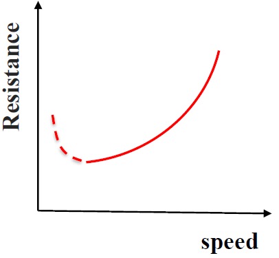
The qualitative speed dependence is illustrated in Figure 7.1: after the low-speed running-resistance minimum, the increasing branch reminds the reader that high-speed operation is dominated by speed-dependent train resistance, especially aerodynamic drag.

Figure 7.1 Schematic relationship between specific running resistance and speed.

Specific resistance is expressed as a force ratio relative to the train weight. For any resistance component \(i\),

\[ w_i = 1000\,\frac{W_i}{P_\mathrm{total}} \quad [‰] \label{eq:specific_resistance_definition} \]

\[ W_i = \frac{w_i}{1000}\,P_\mathrm{total} \label{eq:specific_resistance_force} \]

where \(W_i\) is the resistance force [kN] and \(P_\mathrm{total}\) is the total train weight as a force [kN]. A value of 10 ‰ therefore means a resisting force equal to 1 % of the train weight; for example, a train with \(P_\mathrm{total}=10{,}000\) kN and \(w=10\) ‰ has \(W=100\) kN.

The total specific resistance combines the line and train components:

\[ w_\mathrm{total} = w_\mathrm{curve} + w_\mathrm{gradient} + w_\mathrm{train} \label{eq:overview_total_specific_resistance} \]

\[ W_\mathrm{total} = \frac{w_\mathrm{total}}{1000}\,P_\mathrm{total} \label{eq:overview_total_resistance} \]

The resistance force acts opposite to the direction of motion. Newton's second law can therefore be written as

\[ F - W_\mathrm{total} = m_\mathrm{total} a, \label{eq:tractive_balance_overview} \]

where \(F\) is the tractive force at the wheel–rail contact and \(m_\mathrm{total}\) is the train mass. At constant speed \(a=0\), so the tractive force must balance the total resistance: \(F=W_\mathrm{total}\). For acceleration, \(F>W_\mathrm{total}\); if the tractive force is lower than the total resistance, the train decelerates.

7.2.2 Line Resistance

The two line-resistance mechanisms used in the calculations below are curve resistance and gradient resistance. They are treated separately below because curve resistance is a guidance and contact-friction problem, while gradient resistance is a gravitational force-component problem.

7.2.2.1 Curve Resistance

Curve resistance is the additional running resistance that appears because the wheelsets must be guided through a curved path instead of rolling freely along a tangent track. In Figure 7.2, the leading axle is forced laterally in the curve; when the available play is used up, flange contact and creepage guide the wheelset and create rubbing against the rail. This rubbing, together with small slip in the wheel–rail contact patch, dissipates energy and must be overcome by additional tractive effort.

Figure 7.2 Curve resistance due to wheelset guidance.

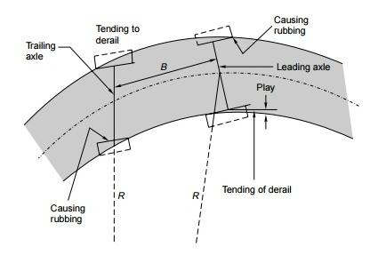
The effect increases as curve radius decreases, because sharper curves require stronger lateral guidance. Wheel conicity can also produce sinusoidal hunting motion on nominally straight track, but in curve-resistance calculations the dominant practical contribution is usually the guidance and flange-friction mechanism in curves.

The specific curve resistance \(w_\mathrm{curve}\) [‰] is calculated using Röckl's empirical formula:

\[ w_\mathrm{curve} = \begin{cases} \dfrac{650}{R - 55} & R \geq 400\,\text{m} \\[8pt] \dfrac{750}{R} & 150\,\text{m} < R < 400\,\text{m} \\[8pt] 5 & R < 150\,\text{m} \end{cases} \label{eq:curve_resistance} \]

where \(R\) is the curve radius in metres. Curve resistance can be neglected when \(R > 1100\) m. In switches and crossings (diverging direction), an additional switch resistance applies.

7.2.2.2 Gradient Resistance

Figure 7.3 illustrates the force balance on an inclined track. The train weight \(P\) acts vertically, but part of this weight acts along the track plane in the downslope direction. This component is the gradient resistance; the tractive effort must at least balance it to maintain constant speed on an upgrade.

Figure 7.3 Gradient resistance on an inclined track.

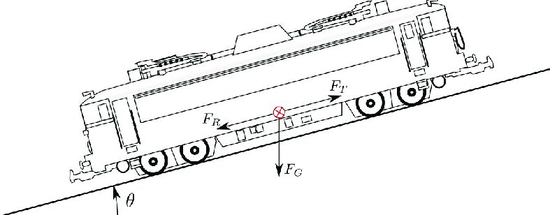
For a gradient angle \(\theta\) (in radians), the required hauling force is:

\[ F_\mathrm{gradient} = P\sin\theta \approx P\theta \label{eq:gradient_force} \]

Railway gradients are normally expressed as a slope \(s\) in ‰. For small angles, \(\sin\theta \approx \tan\theta \approx \theta\), so \(s \approx 1000\theta\). The specific gradient resistance therefore equals the gradient itself:

\[ w_\mathrm{gradient} = s \quad [‰] \label{eq:gradient_resistance} \]

where \(s\) is positive for an upgrade and negative for a downgrade. Large gradients have significant consequences: heavier locomotives, higher energy consumption, reduced payload for freight trains, lower line speeds, longer braking distances, and larger signalling block lengths.

7.2.3 Train Resistance

Train resistance (also called basic resistance) is the running resistance associated with the vehicle itself rather than with the route alignment. Figure 7.4 shows the main mechanisms. Bearing and traction-system resistance come from mechanical losses in the rotating components and drive equipment. Rolling resistance is produced by deformation in the wheel–rail contact and by local irregularities such as rail joints. Dynamic resistance represents energy dissipated as vibration within the vehicle and the wheel–rail system. Aerodynamic resistance is caused by pressure drag at the front of the train and skin friction along the train body; its relative importance grows rapidly with speed.

Figure 7.4 Train-resistance mechanisms.

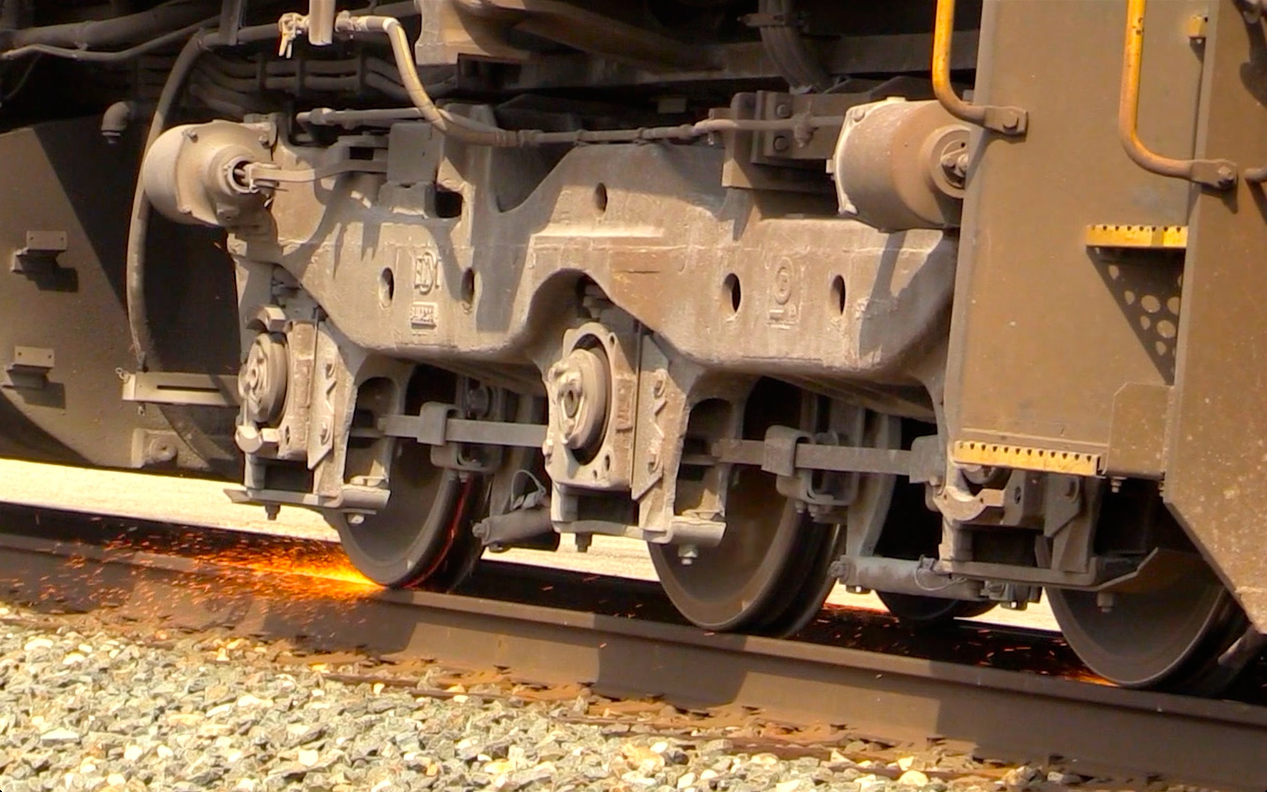
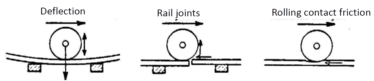
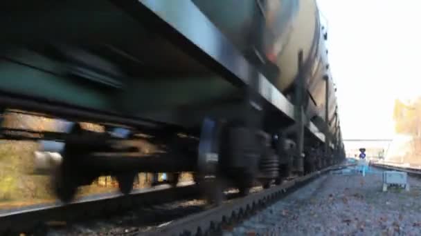
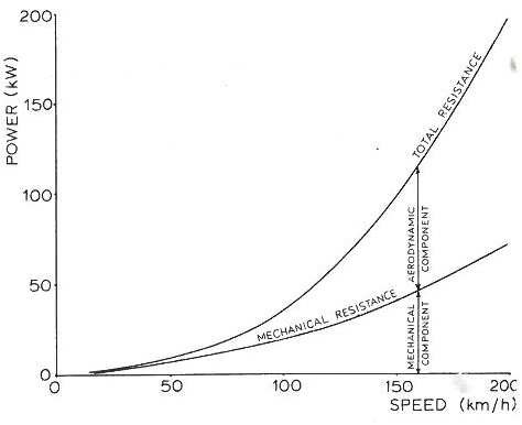
The running resistance of a train is typically only 1.5–2 ‰ of train weight at low to moderate speed, rising with aerodynamic drag at high speed. This is far lower than for road vehicles, primarily due to the small steel-on-steel rolling losses [124].

7.2.3.1 Train Resistance Estimation

The total specific train resistance \(w_\mathrm{train}\) [‰] is approximated by:

\[ w_\mathrm{train} = a + bv + cv^2 \label{eq:train_resistance} \]

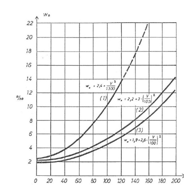
where \(v\) is the speed in km/h and \(a\), \(b\), \(c\) are empirically determined coefficients [124]. The term \((a + bv)\) represents rolling and bearing resistance; \(cv^2\) represents aerodynamic resistance. Figure 7.5 gives typical empirical specific-resistance curves versus speed for different train types.

Figure 7.5 Typical specific train resistance vs. speed for three train generations: (1) older locomotive train, (2) newer locomotive train, (3) modern motor unit train.

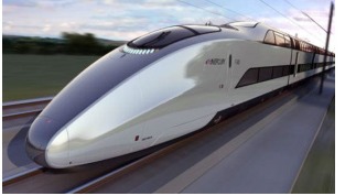
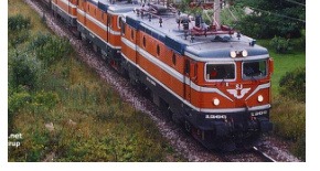
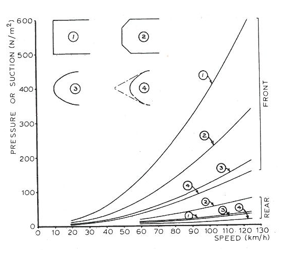
Aerodynamic resistance is strongly affected by the shape of the train front and body cross-section, not only by speed. Figure 7.6 compares a streamlined beak-like form with a slender high-speed train nose and a flatter locomotive front. The kingfisher-like beak in Figure 7.6a is a useful aerodynamic analogy: a long, tapered nose displaces the air more gradually and reduces abrupt pressure build-up. By contrast, the flatter front in Figure 7.6c gives a larger pressure difference and stronger flow separation. This is why the slender nose shape in Figure 7.6b becomes an important design parameter for high-speed trains, where the power needed to overcome aerodynamic resistance is approximately proportional to \(v_r^3\) (relative wind speed cubed).

Figure 7.6 Aerodynamic resistance and front-end shape.

7.2.4 Total Resistance

For a train running at constant speed, the resistance that must be balanced by the tractive effort is the sum of the train resistance and the line resistance. It can be written first as a specific resistance in ‰:

\[ w_\mathrm{total} = w_\mathrm{train} + w_\mathrm{curve} + w_\mathrm{gradient} \label{eq:total_resistance} \]

Here, \(w_\mathrm{train}\) is the basic running resistance of the vehicle, including rolling, bearing, dynamic, and aerodynamic effects. The terms \(w_\mathrm{curve}\) and \(w_\mathrm{gradient}\) describe the additional resistance caused by curves and gradients along the line.

The corresponding total resistance force is obtained by multiplying the specific resistance by the train weight force:

\[ W_\mathrm{total} = \frac{w_\mathrm{total}}{1000}\,P \label{eq:total_resistance_force} \]

In this conversion, \(P\) is the train weight expressed as a force, and \(1\) ‰ corresponds to \(1/1000\) of that weight force. Thus, \(W_\mathrm{total}\) is the force that the locomotive must overcome to maintain constant speed; additional tractive effort is required when the train accelerates. In practice, this resistance calculation is used together with the tractive-effort limits introduced in Section 7.3.

7.3 Tractive Forces

Tractive force is the useful force transferred from the powered wheels to the rail. Its practical value is governed both by installed power and by available adhesion at the wheel–rail contact.

7.3.1 Specific Tractive Force

The specific tractive force \(f\) [‰] is the tractive force \(F\) [kN] per unit train weight \(P_\mathrm{total}\) [kN]:

\[ f = 1000\,\frac{F}{P_\mathrm{total}} \label{eq:specific_tractive} \]

This value is most useful when it is compared with the total specific resistance of the route. At constant speed, the available specific tractive force must be at least as large as the sum of train, curve, and gradient resistance.

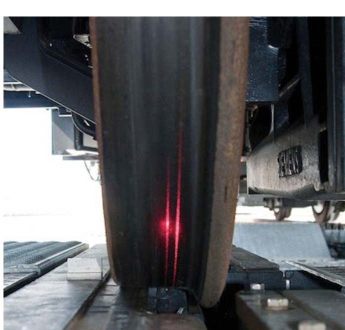
Figure 7.7 connects the specific tractive-force definition to the wheel–rail contact patch: the force can only be transmitted if the tangential contact force remains below the adhesion available from the normal wheel load.

Figure 7.7 Wheel–rail contact patch: available adhesion at this interface limits the transferable tractive force.

7.3.2 Limits on Tractive Effort

The maximum tractive effort is limited by two factors:

1. Available power

The traction system can only deliver a finite rate of mechanical work. Since power is force multiplied by speed, the tractive force that can be sustained by a given installed power decreases as speed increases:

\[ F_\mathrm{power} = \frac{P_\mathrm{engine}}{v} \label{eq:power_limit} \]

where \(P_\mathrm{engine}\) is the engine power [kW] and \(v\) is the speed [m/s]. With these units, \(F_\mathrm{power}\) is obtained in kN.

2. Available adhesion force

Even when sufficient engine power is available, the powered wheels cannot transmit more tangential force than the wheel–rail contact can support without slip. The adhesion limit is therefore proportional to the normal load carried by the driven wheels:

\[ F_\mathrm{adh} = \mu \cdot Q_\mathrm{adh} \label{eq:adhesion_force} \]

where \(\mu\) is the wheel–rail adhesion coefficient and \(Q_\mathrm{adh}\) is the total vertical load carried by the driven wheels or driven axles considered in the calculation. The transferable tractive effort is governed by the lower of the power limit and the adhesion limit:

\[ F_\mathrm{max} = \min(F_\mathrm{power}, F_\mathrm{adh}) \label{eq:max_tractive_effort} \]

The adhesion coefficient for a steel wheel on a steel rail ranges from about 0.10 (wet, contaminated) to 0.40 (dry, clean), and generally decreases with speed.

The speed dependence is compared in Figure 7.8: all the empirical curves reduce the available adhesion as speed increases, and the lower curves represent the reduced margin under damp, contaminated, or otherwise poor rail conditions.

Figure 7.8 Indicative adhesion coefficient μ for dry, damp and poor rail conditions as a function of speed.

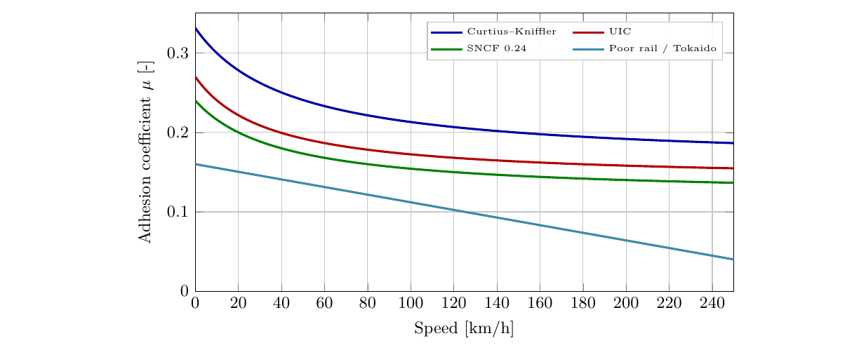
Common adhesion coefficient formulas:

• UIC: \(\mu = 0.139 + 4.48/(v + 34.2)\)

• Curtius–Kniffler: \(\mu = 0.161 + 7.5/(v + 44)\)

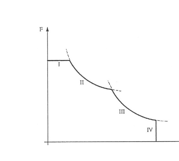
where \(v\) is in km/h. Combining the adhesion limit with installed power gives the staged tractive-effort characteristic in Figure 7.9: low speed is adhesion-limited, then falling adhesion and finally the engine power limit control the available force.

Figure 7.9 Tractive effort characteristic of a locomotive showing four stages: (I) upper adhesion limit, (II) falling adhesion with increasing speed, (III) power limit of the engine, (IV) maximum speed.

Worked example: wagon capacity on a gradient.

The resistance equations and tractive-effort limits are normally used together. Consider an EL 18 locomotive with mass \(M_\mathrm{loc}=82.2\) t hauling loaded freight wagons at \(v=140\) km/h on straight track with a gradient of \(s=6\) ‰. Assume that the available tractive effort at this speed is \(F_\mathrm{avail}=150\) kN. The locomotive basic resistance is estimated as

\[ w_{\mathrm{train,loc}} = 2.2 + 3\left(\frac{v}{100}\right)^2 = 2.2 + 3(1.4)^2 = 8.08\,‰, \]

and the loaded wagons are taken as \(w_{\mathrm{train,wag}}=5\,‰\).

At constant speed, the available tractive effort must balance the total resistance. Using Equations 7.10 and 7.11, and noting that there is no curve resistance on tangent track, the force balance may be written as

\[ F_\mathrm{avail} = \frac{9.81}{1000} \left[ (w_{\mathrm{train,loc}}+s)M_\mathrm{loc} +(w_{\mathrm{train,wag}}+s)M_\mathrm{wag} \right], \]

where masses are in tonnes and the result is in kN. Solving for the maximum loaded wagon mass gives

\[ \begin{aligned} M_\mathrm{wag,max} &= \frac{F_\mathrm{avail}\,1000/9.81 -(w_{\mathrm{train,loc}}+s)M_\mathrm{loc}} {w_{\mathrm{train,wag}}+s}\\ &= \frac{150\,000/9.81-(8.08+6)\cdot82.2}{5+6}\\ &\approx 1285\,\mathrm{t}. \end{aligned} \]

If each wagon has two bogies with two axles per bogie and a maximum axle load of 18 t, one fully loaded wagon has a gross mass of \(4\cdot18=72\) t. The locomotive can therefore pull

\[ n_\mathrm{full} = \left\lfloor \frac{1285}{72} \right\rfloor = 17 \]

fully loaded wagons under these assumptions. Equivalently, about 18 wagons could be used if the average loaded mass per wagon is kept slightly below the 72 t gross-wagon-mass limit implied by the 18 t-per-axle limit.

7.4 Train Dynamic Modelling

Understanding the dynamic behaviour of a railway vehicle is essential for the track engineer: vehicle dynamics determine the forces that the vehicle exerts on the track, and track irregularities are the primary source of dynamic excitation. The simplified modelling framework in this section draws on the rail-vehicle dynamics treatment by Knothe and Stichel [119], with notation adapted for the compendium.

7.4.1 Degrees of Freedom of a Railway Vehicle Body

A rigid railway vehicle body moving along the track has six degrees of freedom (DOF) relative to the track geometry [113, 60]. Figure 7.10 illustrates the three translational motions and the three rotations of the vehicle body. The notation for these motions is used consistently in the following dynamic models.

Figure 7.10 Six rigid-body degrees of freedom of a railway vehicle body.

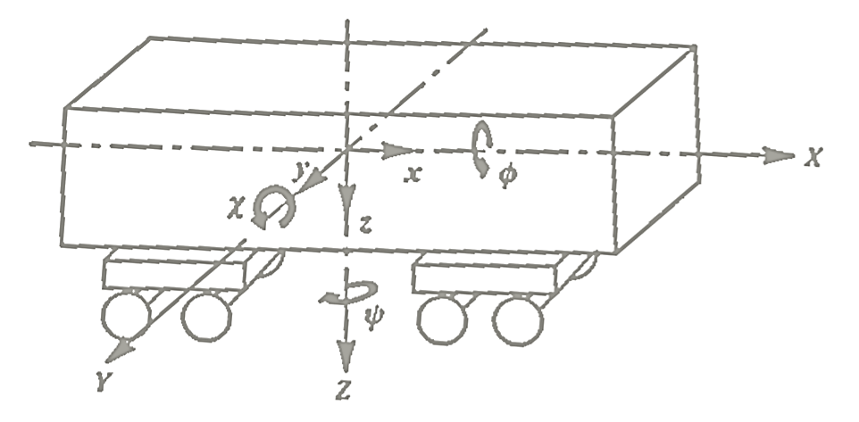
Relative motion	Symbol	Notation
Translation in direction of travel	\(x\)	Longitudinal
Translation transverse (parallel to track plane)	\(y\)	Lateral
Translation perpendicular to track plane	\(z\)	Vertical (bounce)
Rotation about the longitudinal axis	\(\phi\)	Roll / sway
Rotation about the transverse axis	\(\theta\)	Pitch
Rotation about the vertical axis	\(\psi\)	Yaw

Table 7.1 Six rigid-body degrees of freedom of a railway vehicle body relative to the track.

For practical dynamic analysis it is often sufficient to model only vertical motion (bounce) and pitch, since lateral modes are analysed separately. The analysis frequency range of interest is typically 0–150 Hz for structural vehicle dynamics.

7.4.2 Equations of Motion: 1-DOF Model

The simplest model of a vehicle running over a track irregularity is a one-dimensional, single degree-of-freedom (1-DOF) mass-spring-damper system [113]. The suspended vehicle mass \(m\) is the dynamic degree of freedom. The wheel or unsprung mass \(m_w\) is assumed to follow the track irregularity \(z_t(s)\) and is retained in the contact-force calculation because its vertical acceleration contributes directly to the rail load. Figure 7.11 sets up this modelling assumption. In the left-hand sketch, the vehicle body mass is connected to the wheel or unsprung mass by suspension stiffness \(k\) and damping \(c\), while the wheel follows the prescribed track profile \(z_t(s)\). The right-hand free-body sketch shows the same model in force form: the spring force \(F_{k,d}\) and damping force \(F_c\) act through the suspension, and the dynamic contact force \(Q_d\) acts at the wheel–rail interface.

Figure 7.11 One-dimensional 1-DOF train–track interaction model.

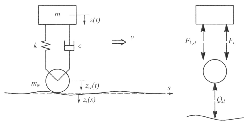
From equilibrium of the vehicle body and the wheelset:

\[ \begin{aligned} m\ddot{z} &= -F_{k,d} - F_c \label{eq:eom_body} \\ m_w \ddot{z}_w &= F_{k,d} + F_c - Q_d \label{eq:eom_wheel} \end{aligned} \]

where the spring force and damping force are:

\[ \begin{aligned} F_{k,d} &= k(z - z_w) \label{eq:spring_force} \\ F_c &= c(\dot{z} - \dot{z}_w) \label{eq:damping_force} \end{aligned} \]

Substituting Equations (7.18) and (7.19) into Equations (7.16) and (7.17):

\[ \begin{aligned} m\ddot{z} + c(\dot{z} - \dot{z}_w) + k(z - z_w) &= 0 \label{eq:eom_body2} \\ m_w\ddot{z}_w - c(\dot{z} - \dot{z}_w) - k(z - z_w) &= -Q_d \label{eq:eom_wheel2} \end{aligned} \]

The track irregularity \(z_t(s)\) is a function of position \(s\) along the track. As the vehicle travels at constant speed \(v\), the position at time \(t\) is \(s(t) = s_0 + vt\), so the wheel displacement, velocity, and acceleration are:

\[ \begin{aligned} z_w &= z_t[s(t)] \\ \dot{z}_w &= z_t'v \\ \ddot{z}_w &= z_t''v^2 \end{aligned} \]

Substituting into Equation (7.21), the dynamic contact force \(Q_d\) (the additional force above the static wheel load \(Q_0\)) is:

\[ Q = Q_0 + Q_d = (m + m_w)g - m\ddot{z} - m_w z_t''v^2 \label{eq:contact_force_1dof} \]

This shows that contact force variations are driven by (i) vehicle body acceleration \(\ddot{z}\) (suspension response) and (ii) wheel acceleration \(z_t''v^2\) (unsprung mass following the irregularity profile at speed \(v\)).

7.4.3 Equations of Motion: 2-DOF Model

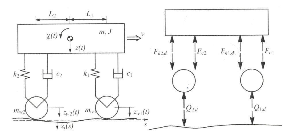
A more realistic model includes two wheelsets (mass \(m_w\) each) at distances \(L_1\) and \(L_2\) from the body centre of mass, with independent primary suspensions \((k_1, c_1)\) and \((k_2, c_2)\) [113]. Figure 7.12 illustrates this extension of the 1-DOF model. The vehicle body has mass \(m\) and pitch moment of inertia \(J\); the generalised coordinates are the vertical displacement \(z\) and the pitch angle \(\chi\). The two wheelsets follow the track profile at positions \(z_{w1}(t)\) and \(z_{w2}(t)\), while the dynamic wheel–rail contact forces are \(Q_{1,d}\) and \(Q_{2,d}\). The free-body sketch on the right defines the force directions used in the equilibrium equations below.

Figure 7.12 Two-wheelset 2-DOF train–track interaction model.

Force and moment equilibrium for the vehicle body:

\[ \begin{aligned} m\ddot{z} &= -F_{k1,d} - F_{c1} - F_{k2,d} - F_{c2} \label{eq:2dof_force}\\ J\ddot{\chi} &= -F_{k1,d}L_1 - F_{c1}L_1 + F_{k2,d}L_2 + F_{c2}L_2 \label{eq:2dof_moment} \end{aligned} \]

Wheelset equations of motion:

\[ \begin{aligned} m_w\ddot{z}_{w1} &= F_{k1,d} + F_{c1} - Q_{1,d} \label{eq:2dof_ws1}\\ m_w\ddot{z}_{w2} &= F_{k2,d} + F_{c2} - Q_{2,d} \label{eq:2dof_ws2} \end{aligned} \]

In matrix form, the equations of motion of the vehicle body become:

\[ \begin{bmatrix} m & 0 \\ 0 & J \end{bmatrix} \begin{Bmatrix} \ddot{z} \\ \ddot{\chi} \end{Bmatrix} + \mathbf{C} \begin{Bmatrix} \dot{z} \\ \dot{\chi} \end{Bmatrix} + \mathbf{K} \begin{Bmatrix} z \\ \chi \end{Bmatrix} = \mathbf{f}(z_{w1}, z_{w2}) \label{eq:matrix_eom} \]

where \(\mathbf{C}\) and \(\mathbf{K}\) are the damping and stiffness matrices incorporating the suspension parameters, and \(\mathbf{f}\) is the excitation vector driven by the two wheelset positions. The total contact forces on wheelsets 1 and 2, including the static wheelset weight terms, are:

\[ \begin{aligned} Q_1 &= \left(m_w + \frac{mL_2}{L_1+L_2}\right)g - m_w\ddot{z}_{w1} - c_1(\dot{z}+\dot{\chi}L_1-\dot{z}_{w1}) - k_1(z+\chi L_1-z_{w1}) \label{eq:q1_2dof}\\ Q_2 &= \left(m_w + \frac{mL_1}{L_1+L_2}\right)g - m_w\ddot{z}_{w2} - c_2(\dot{z}-\dot{\chi}L_2-\dot{z}_{w2}) - k_2(z-\chi L_2-z_{w2}) \label{eq:q2_2dof} \end{aligned} \]

Here the body coordinate \(z\) is measured at the centre of mass. Positive rotation \(\chi\) increases the displacement at wheelset 1 and decreases it at wheelset 2. The distances from the centre of mass to wheelsets 1 and 2 are \(L_1\) and \(L_2\).

7.4.4 Symmetric Undamped Natural Frequencies

The 2-DOF model above can be reduced to a simple hand calculation when the vehicle is symmetric and damping is neglected. Let \(k_1=k_2=k\), \(L_1=L_2=L\), \(c_1=c_2=0\), and set the prescribed track input to zero for free vibration. The equations then become

\[ \begin{bmatrix} m & 0 \\ 0 & J \end{bmatrix} \begin{Bmatrix} \ddot{z} \\ \ddot{\chi} \end{Bmatrix} + \begin{bmatrix} 2k & 0 \\ 0 & 2kL^2 \end{bmatrix} \begin{Bmatrix} z \\ \chi \end{Bmatrix} = \begin{Bmatrix} 0 \\ 0 \end{Bmatrix}. \label{eq:symmetric_undamped_eom} \]

The bounce and pitch motions are uncoupled in this special case. The eigenvalue problem \(\mathbf{K}\boldsymbol{\phi}=\omega^2\mathbf{M}\boldsymbol{\phi}\) therefore gives

\[ \omega_z=\sqrt{\frac{2k}{m}}, \qquad \omega_\chi=\sqrt{\frac{2kL^2}{J}}, \qquad f=\frac{\omega}{2\pi}. \label{eq:symmetric_undamped_frequencies} \]

For example, with \(m=32\,000\) kg, \(J=900\,000\) kg m\(^2\), \(k=850\) kN/m and \(L=8\) m:

\[ f_z=\frac{1}{2\pi}\sqrt{\frac{2\cdot850\,000}{32\,000}} =1.16\,\mathrm{Hz}, \qquad f_\chi=\frac{1}{2\pi}\sqrt{\frac{2\cdot850\,000\cdot8^2}{900\,000}} =1.75\,\mathrm{Hz}. \]

These values are close to typical low-frequency carbody bounce and pitch modes. If the vehicle is not symmetric, or if damping and different front/rear suspension properties are included, the off-diagonal terms no longer vanish and the full matrix eigenvalue problem must be solved.

7.4.5 Eigenvalues and Eigenmodes

Eigenvalue analysis (free vibration with zero damping) reveals the natural frequencies and mode shapes of the vehicle system when the bodies are treated as rigid [113]. Figure 7.13 illustrates the carbody, secondary suspension, bogie frame, primary suspension, and wheelset layout behind the main rigid-body mode families. For a bogie vehicle with two bogies, each with two wheelsets, the carbody modes are mainly bounce, pitch, yaw, and sway, while higher-frequency modes are associated with bogie and wheelset motion.

Figure 7.13 Bogie passenger vehicle mode families.

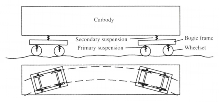
The typical frequency ranges for these mode families are summarised in Table 7.2.

Mode	Typical frequency	Description
Lower sway	\(\approx 0.6\) Hz	Body rolling about longitudinal axis (low secondary suspension)
Body bounce	\(\approx 1.1\) Hz	Body vertical translation
Body pitch	\(\approx 1.35\) Hz	Body rotation about transverse axis
Body yaw	\(\approx 1.3\) Hz	Body rotation about vertical axis
Upper sway	\(\approx 1.8\) Hz	Body rolling (high secondary suspension)
1st bogie kinematic	\(\approx 4.5\) Hz	Wheelset hunting on 1st bogie
2nd bogie kinematic	\(\approx 4.6\) Hz	Wheelset hunting on 2nd bogie
Bogie longitudinal	\(\approx 9.5\) Hz	Bogie fore-aft vibration

Table 7.2 Typical eigenfrequencies for a bogie passenger vehicle [113, 4].

Knowing these natural frequencies is critical for the track engineer: track irregularities at the corresponding excitation wavelengths can excite resonance, leading to large dynamic contact forces. For instance, a body bounce mode at 1.1 Hz excited at 100 km/h corresponds to an irregularity wavelength of \(\lambda = v/f = 100\,000/(3600 \times 1.1) \approx 25\,\mathrm{m}\), a wavelength controlled by tamping and subgrade maintenance.

7.5 Track Dynamics

Track dynamics extends the static load models by considering excitation frequency and resonance. This is essential when speed, wheel defects, or short-wavelength irregularities amplify forces.

7.5.1 Vibration Excitation Sources

Track dynamic forces are excited by geometric irregularities in the wheel and rail surfaces. The excitation frequency \(f\) from a periodic defect of wavelength \(\lambda\) at speed \(v\) is:

\[ f = \frac{v}{3.6 \cdot \lambda} \label{eq:excitation_frequency} \]

(with \(v\) in km/h and \(\lambda\) in metres). This formula can be applied to calculate excitation frequencies from rail corrugations, wheel flats, sleeper passing, and other periodic track features.

7.5.2 Track Natural Frequencies

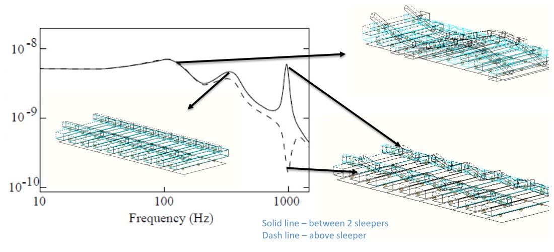
The track has three characteristic resonance frequency ranges (track receptance peaks). The receptance plot in Figure 7.14 illustrates how these ranges appear in the frequency response of the rail: the lower-frequency peak involves the rail and sleepers moving on the ballast, the middle range is governed by the railpad support, and the high-frequency peak is the pinned–pinned rail mode between sleepers.

1. 40–140 Hz: Rail and sleepers bouncing together on the ballast

2. 100–500 Hz: Rail bouncing on the railpads (pad resonance)

3. 850–1200 Hz: Pinned-pinned resonance, where the wavelength equals twice the sleeper spacing

Figure 7.14 Track receptance peaks and characteristic vibration shapes.

7.5.3 Vibration Categories and Their Consequences

Railway vibration problems are usefully separated by frequency range because vehicle stability, track dynamics, rolling noise, and ground-borne vibration involve different mechanisms and mitigation measures.

Category	Typical problem mechanisms	Frequency range [Hz]
Vehicle	Stability, curvature and guidance behaviour, passenger comfort	0–30
Bogie and unsuspended masses	Wheel bearings; operating strength of axles, bearings, brakes, wheelsets and bogie frames	0–200
Wheel and rail running faces	Wheel flats, skid marks, polygonised wheels, wheel corrugation, rail corrugation, joints, badly ground welds and rolling contact fatigue	50–200 for long-wave corrugation; up to 1500 for short-wave defects
Rail components	Rail fatigue, aged rail pads, concrete sleepers, ballast settlement, deterioration of track geometry and subsoil settlement	0–1500
Wheel–rail noise	Rolling noise, impact noise and curve squeal	0–5000
Structure-borne noise and shocks	Shock propagation in the subsoil, bridge vibration, sound emission and structure-borne vehicle-body noise	0–500

Table 7.3 Classification of railway vibration and noise problems by typical frequency range.

Track vibration problems are categorised by frequency [60, 113]:

• 0–30 Hz: Vehicle stability, curvature and guidance behaviour

• 0–200 Hz: Wheel bearings, bogie and unsuspended mass dynamics, wheel flats, polygonised wheels, wheel corrugation, long-wave rail corrugation

• 0–1500 Hz: Short-wave rail corrugation, rail joints, badly ground welds, rolling contact fatigue (head checks, squats) and rail surface defects

High-frequency vibrations at the wheel–rail contact generate noise and can accelerate fatigue damage. Rail grinding (Chapter 16) is the primary maintenance tool to control corrugation and fatigue crack initiation [103, 122].

7.6 Train–Track Interaction

The train and the track interact dynamically: vehicle motions excite the track, and track irregularities and stiffness variations excite the vehicle. This section covers the principal phenomena at the train–track interface that arise from this coupling.

7.6.1 Sleeper Passing Frequency

The rail is supported discretely at each sleeper, not continuously. As a wheel rolls along the rail, it encounters a periodic variation in support stiffness with a spatial period equal to the sleeper spacing \(l\). This generates a periodic excitation force at the sleeper passing frequency [151, 113]:

\[ f_\mathrm{sp} = \frac{v}{l} \label{eq:sleeper_passing} \]

where \(v\) is the wheel velocity [m/s] and \(l\) is the sleeper spacing [m]. For a typical sleeper spacing of \(l = 0.60\) m and a speed of \(v = 140\) km/h (\(\approx 38.9\) m/s):

\[ f_\mathrm{sp} = \frac{38.9}{0.60} \approx 65\,\text{Hz} \]

This frequency is far below the pinned–pinned rail resonance range (850–1200 Hz), but it lies within the ballast-bounce and lower wheelset-mode range. If the sleeper passing frequency coincides with a wheelset structural eigenmode (e.g. a bending mode of the wheelset at 60–80 Hz), resonance can develop, producing repeated contact excitation at each sleeper location. This is one mechanism associated with short-pitch rail corrugation [101, 151].

7.6.2 Frequency-Dependent Track Stiffness

Track stiffness is not a static quantity: it varies with excitation frequency due to the inertia of the rail, sleeper, and ballast [151, 60]. Measurements show that:

• Vertical stiffness increases with frequency, from static values of \(\approx 30\)–60 kN/mm to higher apparent stiffness at frequencies above \(\sim 100\) Hz.

• Concrete sleeper track (stiffer) shows higher damping coefficients than wooden sleeper track in the relevant frequency range, though damping results carry large uncertainties.

• Lateral stiffness is substantially lower than vertical stiffness:

• Wooden sleepers with base plate and rail spike: 5–10 MN/m

• Concrete sleepers with elastic fastenings: 15–20 MN/m

Knowledge of lateral flexibility remains limited compared to vertical stiffness, yet it is important for lateral force transfer and wheel–rail guidance behaviour discussed in Chapter 8.

7.6.3 Influence of Suspension on Curving

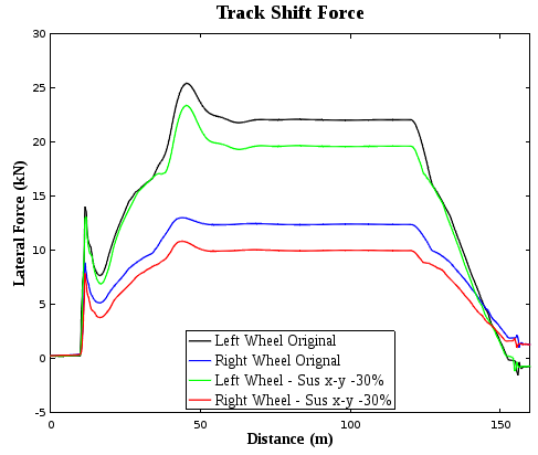
In curves, the primary suspension stiffness governs the steering of the vehicle. Figure 7.15 shows the resulting lateral track-shift force: when the wheelsets can rotate more nearly towards the radial direction, the angle of attack and the lateral force acting on the track are reduced.

Figure 7.15 Lateral track-shift force during curving.

The practical consequences are:

• A rigid-frame vehicle (single suspension level) has high bogie stiffness and cannot steer easily into curves, resulting in high lateral forces, poor curving behaviour, and a rough ride.

• A bogie vehicle (two suspension levels: primary between wheelset and bogie, secondary between bogie and body) has softer primary suspension that allows the wheelsets to steer into the curve, reducing lateral forces.

• Generally, softer longitudinal and lateral primary suspension improves curving performance. This is in tension with the high-speed stability requirement, so suspension design is a compromise between curving and stability. Wheelset hunting and limit-cycle behaviour are treated with wheel–rail guidance in Chapter 8.

The curving performance directly affects track maintenance: good curving (low lateral force) reduces gauge widening, repeated flange contact and maintenance demand in tight curves [65, 124].

7.7 Chapter Summary

Resistance and traction. Before dynamic vibration is considered, a train must overcome line resistance from curves and gradients and train resistance from rolling, bearing and aerodynamic effects. The total resistance determines the tractive effort required to maintain or increase speed, while adhesion and the locomotive traction system limit what can actually be delivered at the wheel–rail interface. These concepts connect vehicle performance directly to alignment and operating conditions.

Vehicle motion. Railway vehicles do not move only vertically; they heave, pitch, roll, sway, yaw and bounce through the primary and secondary suspension systems. Simplified one- and two- degree-of-freedom models are useful because they show how mass, stiffness and damping control natural frequency and response amplitude. Even when real vehicles are more complex, these simple models explain why suspension tuning and track stiffness strongly influence ride quality and dynamic loading.

Excitation. A track irregularity becomes a dynamic input when the train passes over it, and the excitation frequency is controlled by vehicle speed divided by irregularity wavelength. Sleeper-passing frequency, corrugation wavelength, wheel flats and alignment defects can therefore excite vehicle or track modes if their frequencies fall near a natural frequency. This is why speed increases can change a harmless irregularity into a damaging vibration problem.

Track stiffness. The track is not a rigid foundation: rails, pads, sleepers, ballast and substructure form a layered dynamic system with stiffness and damping that vary with frequency and load level. Too low stiffness can lead to excessive deflection and settlement, while too high stiffness can increase impact forces and vibration transmission. Good track design therefore seeks compatible stiffness rather than simply making every layer as stiff as possible.

Maintenance link. Curving forces, traction limits, resonance, sleeper passing and frequency-dependent support all affect rail wear, ballast degradation, geometry deterioration and passenger comfort. The chapter therefore provides the mechanical bridge between earlier loading chapters and later topics such as wheel–rail interaction, CWR, noise, vibration and maintenance planning.

Assignments

Assignment 1: Dynamic train movement

(a) What are the two primary types of resistance that a train must overcome to start moving or to maintain motion?

(b) The plot below shows typical specific train resistance for an older locomotive train, a newer locomotive train, and a modern motor unit train. Why do older train types normally have higher resistance?

(c) An EL 18 electric locomotive hauls loaded wagons at constant speed \(v=140\) km/h on straight track. The locomotive mass is \(M_\mathrm{loc}=82.2\) t and the starting tractive effort is 275 kN. For the calculation, take the available tractive effort at 140 km/h as 150 kN. The locomotive basic resistance is

\[ w_{\mathrm{train,loc}} = 2.2 + 3\left(\frac{v}{100}\right)^2 \quad [‰], \]

and the specific basic resistance of the wagons is \(w_{\mathrm{train,wag}}=5\) ‰.

(i) Calculate the minimum adhesion coefficient required if the locomotive uses the maximum available tractive effort at the start.

(ii) Calculate the maximum loaded wagon mass that can be pulled by one EL 18 up a gradient of 6 ‰ at 140 km/h. Also determine how many fully loaded wagons can be pulled if each wagon has two bogies with two axles per bogie and a maximum axle load of 18 t.

(iii) How steep can the maximum gradient be when two EL 18 locomotives pull 980 t of loaded wagons at 140 km/h in wet conditions (\(\mu=0.15\))? Assume straight track and constant speed.

Assignment 2: Three-DOF wagon model with traction

A simplified wagon with traction can be modelled as shown below with three generalised coordinates: longitudinal displacement \(x(t)\), vertical displacement \(z(t)\) and pitch angle \(\chi(t)\). The suspended mass is \(m\) and the pitch moment of inertia about its centre of gravity is \(J\). Each wheelset has mass \(m_w\). The primary suspension has stiffness \(k\) and damping coefficient \(c\), and each traction rod has longitudinal stiffness \(k_{tr}\). The distance between the two wheelsets is \(2L\). The nominal height difference between the centre of gravity of the suspended mass and the traction-rod/drawbar level is \(h\).

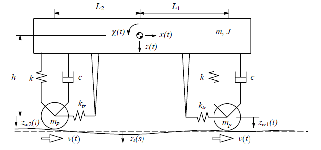
Assume that the wheelsets do not lose contact with the rails. Their prescribed vertical motions are \(z_{w1}(t)\) and \(z_{w2}(t)\). The train speed is \(v(t)=v_0+at\), where \(a\) is constant acceleration, and the vertical track profile is described by \(z_t(s)\). Use the sign convention in the figure: at wheelset 1 the body vertical displacement is \(z-\chi L\), while at wheelset 2 it is \(z+\chi L\).

(a) Derive the three equations of motion for the suspended mass.

(b) Write the resulting mass, damping and stiffness matrices and the load vector in the form \(\mathbf{M}\ddot{\mathbf{q}}+\mathbf{C}\dot{\mathbf{q}}+\mathbf{K}\mathbf{q} =\mathbf{f}(t)\), where \(\mathbf{q}=\{x,z,\chi\}^T\).

(c) Give expressions for the two vertical wheel–rail contact forces \(Q_1\) and \(Q_2\), including the wheelset acceleration terms.

(d) What does pinned–pinned resonance mean in railway track receptance? (Lateral hunting stability and curving behaviour are treated separately in Chapter 8.)

Assignment 3: Track receptance and dynamic response

(a) What does track receptance mean, and why are receptance peaks important for dynamic train–track interaction?

(b) Give three examples of periodic or impulsive excitation sources that can produce large dynamic wheel loads when their forcing frequency approaches a track resonance range.

(c) Explain how a change in train speed can either increase or reduce the dynamic amplification from a given defect wavelength.

Assignment 4: Track resistance

Track shift can occur frequently in tight curves. Suggest at least five remedies that can reduce this problem. At least two suggestions should be from the train or vehicle perspective. Briefly explain why each suggestion helps.

Assignment 5: Resonance and excitation frequency

A train runs at 160 km/h on ballasted track with sleeper spacing \(l=0.60\) m. A short-pitch rail corrugation with wavelength \(\lambda=0.18\) m is also present.

(a) Calculate the sleeper-passing frequency and the corrugation excitation frequency.

(b) State which characteristic track frequency range each excitation is most likely to approach: ballast bounce, railpad resonance, or pinned–pinned rail resonance.

(c) Repeat the calculation for 80 km/h and explain why a speed change can reduce dynamic amplification.

Assignment 6: Vehicle modes and irregularity wavelengths

A vehicle has a vertical carbody mode at approximately 1.1 Hz and a bogie kinematic mode at approximately 4.5 Hz. For a train speed of 100 km/h:

(a) Calculate the track-irregularity wavelength that would excite each mode.

(b) Explain why long-wavelength geometry errors mainly affect vehicle-body motion, while shorter wavelengths can excite bogie and wheelset motion.

(c) Give two examples of track defects or maintenance conditions that can create periodic excitation.