05

Geometric Design of Track Systems

5.1 Introduction

The geometric design of a railway line defines the three-dimensional shape of the track alignment [65, 10, 141]. It determines the allowable speeds, passenger comfort, train stability, track wear rates, and energy consumption of the line. The track alignment is defined within a coordinate system and consists of a horizontal alignment (plan view) and a vertical alignment (longitudinal profile). Together these define every point of the track in space.

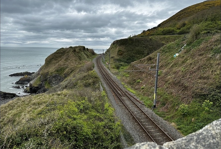
The field photograph below shows the practical setting for this design task: the alignment must follow the terrain while coordinating track curvature, electrification, and the wider railway corridor.

Coastal railway alignment near Bray, Ireland.

The design of track geometry must balance several competing objectives:

• Maximise operating speeds to increase line capacity and reduce travel times

• Minimise the forces on the track and rolling stock to reduce wear and maintenance

• Ensure passenger comfort by limiting lateral and vertical accelerations

• Achieve the design at reasonable construction cost (avoiding excessive earthworks)

• Satisfy safety requirements for all vehicle types that will use the line

The factors that influence the choice of route for a new railway line are geographical, technical, environmental, political, social, and economic. Recent open Norwegian project figures give a useful order of magnitude: complex intercity double-track corridors are often around 1–3 million NOK per route metre, or 1–3 billion NOK per route kilometre, in nominal project-year prices. Drammen–Kobbervikdalen is reported by Bane NOR as about 10 km of new double track with a total cost of 13 billion NOK, corresponding to roughly 1.3 million NOK/m (1.3 billion NOK/km). Sandbukta–Moss–Såstad is also about 10 km and had a proposed cost frame of 27.6 billion NOK after major ground-stability challenges in Moss, corresponding to about 2.8 million NOK/m (2.8 billion NOK/km) [51, 20, 150]. These totals include stations, tunnels, urban works, ground improvement, railway systems, and other project-specific scope. The key point for alignment design is simple: each additional metre of difficult alignment can represent millions of NOK, so geometric choices that control earthwork, tunnelling, bridging, and ground improvement are among the most consequential decisions in railway engineering.

5.1.1 Modelling Assumptions

For the calculations in this chapter, railway alignment is treated as a constrained vehicle–track interaction problem. The horizontal and vertical alignments prescribe the kinematic input to the vehicle, which then responds through suspension motion, wheel–rail contact forces, creep forces, and load transfer. The design parameters in this chapter are therefore not independent: cant, curvature, speed, transition length, vehicle type, axle load, and maintenance condition form a coupled system.

The equations used below are first-order design equations. They assume quasi-static motion, small cant angles, a rigid track plane, and an effective track spacing \(s\) between the rolling-contact points rather than the nominal gauge. These assumptions are appropriate for preliminary design calculations, but not sufficient for final approval of high-speed lines, tilting vehicles, switches and crossings, bridges, or locations with poor track quality. In those cases, vehicle-specific dynamic simulation, route acceptance requirements, and the current Bane NOR technical regulations must govern the final design.

The principal geometric-design variables used in this chapter are defined in Table 5.1.

Symbol	Meaning	Typical unit / note
\(R\)	Horizontal curve radius	m
\(R_v\)	Vertical curve radius	m
\(v\), \(V\)	Train speed	\(v\) in m/s for mechanics equations; \(V\) in km/h for many railway design formulas
\(h\) or \(h_m\)	Applied cant	mm unless inserted in SI equations, where metres must be used
\(I\)	Cant deficiency	mm; equivalent to uncompensated lateral acceleration through \(j_u=gI/s\)
\(I_e\)	Cant excess	mm; governs slow trains and stopping locations
\(L_t\)	Transition-curve length	m
\(x\)	Distance measured from the start of a transition curve	m; \(0 \leq x \leq L_t\)
\(l\)	Vertical-curve tangent length, measured from the vertical intersection point to the start or end of the vertical curve	m
\(s\)	Effective track spacing between rolling-contact points	approximately 1500 mm for standard-gauge design calculations

Table 5.1 Principal geometric-design variables used in this chapter.

5.2 Elements of Track Geometry

Track geometry is built from a small set of horizontal and vertical elements, which are combined to satisfy speed, comfort, terrain, and construction constraints. The same parameters reappear later as field defects in Chapter 15 and as maintenance-limit quantities in Chapter 16.

5.2.1 Overview

The geometry of a railway line consists of horizontal and vertical elements:

Horizontal direction:

1. Straight (tangent track)

2. Circular curve

3. Transition curve (clothoid)

4. Superelevation (cant)

Vertical direction:

1. Gradient (straight gradient line)

2. Vertical curve (parabolic or circular arc)

5.2.2 Straight Track

Straight (tangent) track follows a straight line. It allows:

• Direct, efficient train movement at maximum speed

• Simpler and generally less costly construction and maintenance

• Speed optimisation without the need for cant

There is no centrifugal force on straight track, so passengers experience lateral forces only from track irregularities. From an operations perspective, however, very long and visually monotonous tangents can create low task demand for drivers; train-simulator and EEG studies link such monotonous driving conditions to fatigue, vigilance loss, and performance degradation [61, 121]. Where route constraints allow, this human-factors issue can support introducing gentle curvature rather than using a long tangent purely for its own sake.

5.2.3 Circular Curves

Circular curves are used where the route must change direction. They are characterised by a constant radius \(R\). Tighter radii permit direction changes in shorter distances but limit the permissible speed.

A train travelling at speed \(v\) through a curve of radius \(R\) experiences a centripetal (lateral) acceleration directed towards the centre of curvature [65, 124]:

\[ a_\mathrm{lateral} = \frac{v^2}{R} \label{eq:lateral_acc} \]

This acceleration must be managed through superelevation (cant) and by limiting speed.

5.2.4 Transition Curves

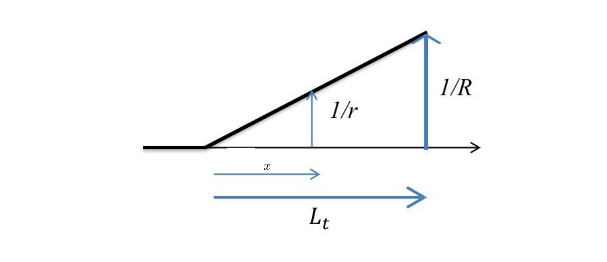
A transition curve (clothoid, also called an easement curve or spiral) provides a gradual change in curvature from zero (on straight track) to \(1/R\) (on a circular curve). The curvature changes linearly with distance along the transition:

\[ \frac{1}{r} = \frac{1}{R} \cdot \frac{x}{L_t}, \qquad 0 \leq x \leq L_t \label{eq:clothoid} \]

where \(x\) is the running distance measured from the start of the transition, \(r\) is the instantaneous radius of curvature at that position, \(R\) is the radius of the circular curve, and \(L_t\) is the total transition length. Thus \(x=0\) gives zero curvature, while \(x=L_t\) gives the circular-curve curvature \(1/R\). Other transition-curve forms exist, but clothoids are generally preferred in railway design because their curvature changes linearly with distance and can therefore be coordinated directly with cant and cant-deficiency ramps. The geometric idea is to let the track leave the tangent gradually and approach the circular curve without an abrupt change in curvature (Figure 5.1).

Figure 5.1 Clothoid transition: curvature increases linearly from zero to 1/R over L_t.

Transition curves serve three purposes:

• Gradually introduce lateral forces as the train enters the curve (passenger comfort)

• Provide the distance over which cant is ramped up from zero to the full value (track geometry)

• Reduce dynamic forces on the track by avoiding abrupt curvature changes (maintenance)

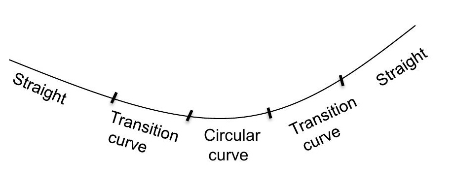
A complete horizontal alignment therefore has a clear sequence: tangent track, transition curve, circular curve, transition curve, and tangent track again (Figure 5.2).

Figure 5.2 Typical horizontal alignment with tangent track, transition curves, and a circular curve.

5.3 Superelevation (Cant)

Cant is one of the key links between geometry and vehicle dynamics, because it determines how much of the centrifugal effect is balanced in curves.

5.3.1 Definition and Purpose

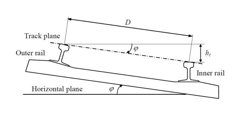
Superelevation (overhøyde), commonly called cant and denoted \(h\), is the difference in height between the outer and inner rails in a curve. The outer rail is raised so that the resultant of the train weight and the centrifugal force acts more nearly perpendicular to the track plane, reducing the lateral force on the wheels and improving passenger comfort. The required cant is selected from the curve radius and design speed so that gravitational and centrifugal effects are balanced as closely as practical for the traffic using the line. Correct cant design improves comfort and reduces wheel–rail wear, while excessive or insufficient cant must be checked through the cant deficiency and cant excess limits.

In geometric terms, cant is the rail-height difference that creates the tilted track plane in a curve (Figure 5.3).

Figure 5.3 Superelevation (cant) in curved track.

5.3.2 Equilibrium Speed and Theoretical Cant

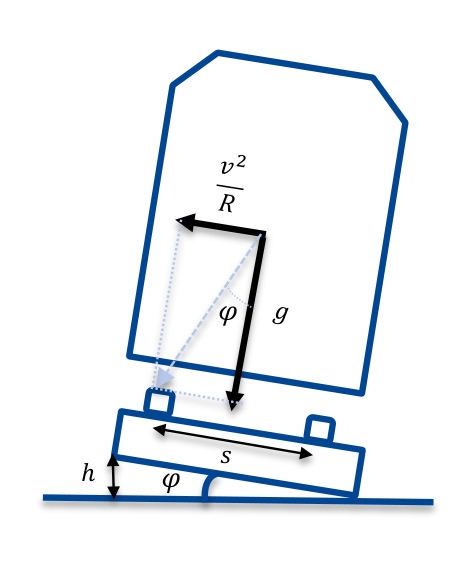
When a train travels at the equilibrium speed \(v_\mathrm{eq}\), the cant exactly balances the centrifugal force and there is no net lateral force on the passengers. The equilibrium condition for small cant angles (so that \(\cos\varphi \approx 1\) and \(\tan\varphi \approx h/s\)) gives:

\[ \frac{v^2}{R} = \frac{g \cdot h}{s} \label{eq:equilibrium} \]

Solving for the equilibrium speed:

\[ v_\mathrm{eq} = \sqrt{\frac{R \cdot g \cdot h}{s}} \label{eq:veq} \]

where \(s = 1500\) mm is the effective track spacing [10, 88] (centre-to-centre distance between rolling-contact points, slightly wider than the nominal gauge of 1435 mm), and \(g = 9.81\) m/s\(^2\). In Eqs. 5.3–5.5, \(v\) is in m/s and the lengths \(h\) and \(s\) must be inserted in consistent units; for SI calculations both are normally converted to metres. The theoretical cant \(h_\mathrm{th}\) required for a given speed is:

\[ h_\mathrm{th}(v) = \frac{s \cdot v^2}{g \cdot R} \label{eq:theoretical_cant} \]

If \(h_\mathrm{th}\) is expressed in millimetres and speed is expressed in km/h, the same relationship is often written in the compact railway form:

\[ h_\mathrm{th}\,[\mathrm{mm}] \approx 11.8\,\frac{V^2}{R} \label{eq:theoretical_cant_kmh} \]

where \(V\) is in km/h and \(R\) is in metres. The coefficient 11.8 follows from \(s \approx 1500\) mm and \(g = 9.81\) m/s\(^2\). At equilibrium speed, the canted track plane balances the lateral effect of motion through the curve (Figure 5.4).

Figure 5.4 A train travelling at equilibrium speed in a curve.

5.3.3 Cant Deficiency

When a train travels at a speed higher than the equilibrium speed, the applied cant is insufficient to fully compensate the centripetal acceleration. The remaining uncompensated lateral acceleration is experienced as a lateral force pushing passengers to the outside of the curve. The cant deficiency \(I\) is:

\[ I = h_\mathrm{th}(v_\mathrm{max}) - h \label{eq:cant_deficiency} \]

The uncompensated lateral acceleration is:

\[ j_u = \frac{v^2}{R} - \frac{g \cdot h}{s} = \frac{g \cdot I}{s} \label{eq:uncompensated_acceleration} \]

The maximum allowable speed in a curve is set by the maximum permitted cant deficiency [10] \(I_\mathrm{max}\):

\[ v_\mathrm{max} = \sqrt{\frac{g}{s}(h + I_\mathrm{max}) \cdot R} \label{eq:vmax_I} \]

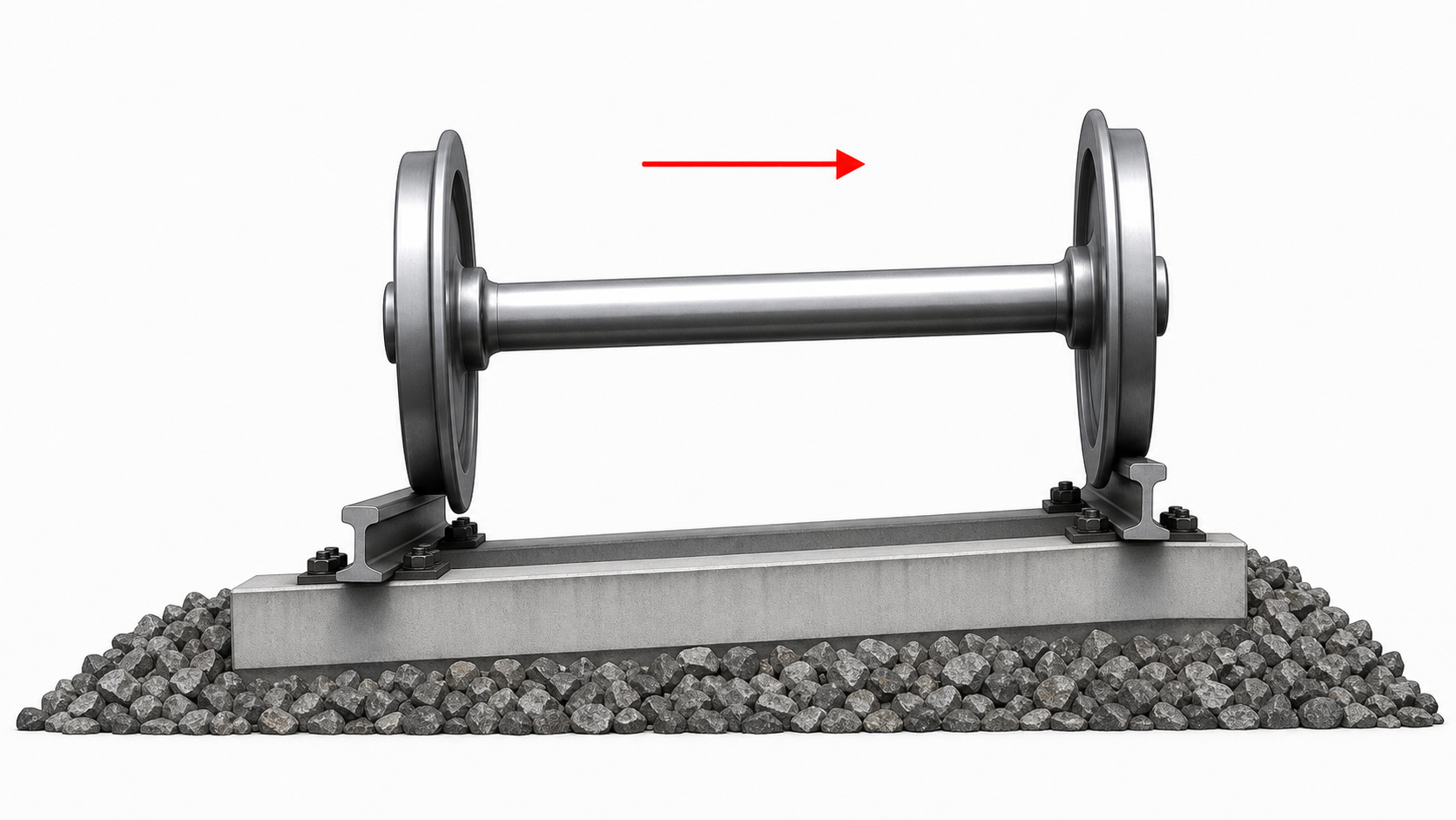
For trains running above the equilibrium speed, the key quantity is the missing cant: the gap between the actual applied cant and the larger theoretical cant required to fully balance the higher speed. At the wheel–rail contact level, the same imbalance can be visualised as a wheelset tendency toward the outer rail (Figure 5.5).

Figure 5.5 Cant deficiency: wheelset bias toward the outer rail.

The maximum speed can be derived from Newton's second law applied to the lateral direction. In a curve of radius \(R\) at speed \(v\), a passenger experiences the lateral uncompensated acceleration \(j_u\):

\[ j_u = \frac{v^2}{R} - \frac{g \cdot h}{s} \label{eq:lateral_accel} \]

Setting \(j_u \leq j_{u,\mathrm{max}}\) and solving for \(v\):

\[ v_\mathrm{max} = \sqrt{\left(\frac{g \cdot h}{s} + j_{u,\mathrm{max}}\right) R} \label{eq:vmax_accel} \]

Since the cant deficiency is related to the uncompensated acceleration by \(I_\mathrm{max} = s \cdot j_{u,\mathrm{max}} / g\), this can equivalently be written as Eq. 5.9:

\[ v_\mathrm{max} = \sqrt{\frac{g\,(h + I_\mathrm{max})}{s} \cdot R} \]

5.3.3.1 Cant Deficiency Limits

Maximum cant deficiency limits are set by standards to ensure wheel/rail safety and passenger comfort:

• New lines and line relocations: typically 100 mm for \(R \leq 600\) m and 130 mm for \(R > 600\) m in Bane NOR technical regulations.

• Existing conventional lines: limits may be 100–150 mm, depending on radius, superstructure class, switches, bridges, and the approved vehicle category.

• Existing lines with approved tilting or "plus" rolling stock: higher vehicle-specific values may be permitted, but they require explicit approval and are not general design values.

Passenger comfort is affected by both the magnitude of the lateral acceleration and its duration and frequency [141, 29]. The acceptable uncompensated acceleration depends on journey duration and frequency content. As a practical guide, \(j_u \approx j_{u,t}/1.5\) where \(j_{u,t}\) is the tolerable acceleration for the journey type and duration. Cant-deficiency limits must therefore be interpreted as vehicle- and approval-dependent comfort and safety criteria, not as one universal value.

Vehicle / case	Typical limit or design implication
Freight traffic	Usually the most restrictive case; commonly limited to about 100 mm for ordinary freight operation.
Conventional passenger traffic	Often in the range 100–150 mm, depending on speed, vehicle approval, and comfort requirements.
Tilting passenger trains	Higher values may be permitted because body tilt reduces passenger-perceived lateral acceleration; special approval is required.
Switches, crossings, platforms, and bridges	More restrictive local limits may apply because of wheel unloading, clearance, structural, or comfort constraints.

Table 5.2 Indicative cant-deficiency limits for different vehicle and approval cases. Project design must use the current Bane NOR technical regulations and vehicle approval basis.

Case study: Santiago de Compostela derailment (2013).

On 24 July 2013, an Alvia passenger train derailed on the A Grandeira curve outside Santiago de Compostela, Spain. The official CIAF investigation records emergency braking before signal E7, when the train was travelling at 195 km/h. It entered the curve at 179 km/h and derailed at PK 84+413, 185 m after the curve began. The curve had \(R=402\) m, applied cant \(h=130\) mm, and an 80 km/h speed limit. The report records 80 fatalities and numerous injuries [58]. These values allow the cant deficiency at the derailment speed to be calculated directly.

The accident line had a nominal track gauge of 1668 mm, which is broader than the 1435 mm gauge used on the Norwegian railway network [2, 29]. For this simplified calculation, use \(s=1.668\) m directly in the same equilibrium-cant equation introduced above. First convert the recorded derailment speed:

\[ v = \frac{V}{3.6} = \frac{179}{3.6} = 49.72\,\mathrm{m/s}. \]

The theoretical cant and cant deficiency are then

\[ \begin{aligned} h_\mathrm{th} &= \frac{s v^2}{gR} = \frac{1.668(49.72)^2}{9.81(402)} \approx 1.046\,\mathrm{m} = 1046\,\mathrm{mm},\\ I &= h_\mathrm{th} - h \approx 1046 - 130 = 916\,\mathrm{mm}. \end{aligned} \]

The corresponding uncompensated lateral acceleration is

\[ j_u = \frac{gI}{s} \approx \frac{9.81\times0.916}{1.668} = 5.39\,\mathrm{m/s^2}. \]

This simple estimate is close to the CIAF result of 5.41 m/s\(^2\). The report notes that this was more than eight times the normal 0.65 m/s\(^2\) limit and about 4.5 times the 1.2 m/s\(^2\) value applicable to the accident train [58]. The equilibrium cant of about 1.05 m is a notional force-balance result, not a practicable track cant. The useful engineering result is the approximately 916 mm cant deficiency, which exposes the extreme lateral imbalance at the recorded derailment speed.

5.3.3.2 Tilting Trains

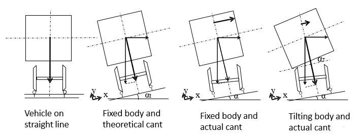
Tilting trains use body tilting mechanisms to compensate for cant deficiency by inclining the car body towards the inside of the curve, effectively adding to the applied track cant from the passengers' perspective. The vehicle-body rotation in Figure 5.7 is the practical expression of this idea: the passenger experiences an effective tilt larger than the track cant alone.

Figure 5.6 Principle of tilting trains.

Two types of tilting mechanisms are used:

• Passive tilting: 2–4\(^\circ\) tilt angle; the body tilts under gravity as the bogie enters the curve

• Active tilting: 6–8\(^\circ\) tilt angle; sensors detect the curve entry and actuators actively tilt the body

Tilting trains can operate faster than non-tilting trains on a given curved alignment because the passengers experience a smaller lateral acceleration. The track and wheel–rail forces, however, are governed by the actual speed, radius, applied cant, and vehicle approval basis; tilting therefore does not remove the need to check cant deficiency, wheel unloading, and track forces.

5.3.4 Cant Excess

When a train travels at a speed below the equilibrium speed, the applied cant is excessive. The cant excess \(I_e\) is:

\[ I_e = h - h_\mathrm{th}(v_\mathrm{min}) \label{eq:cant_excess} \]

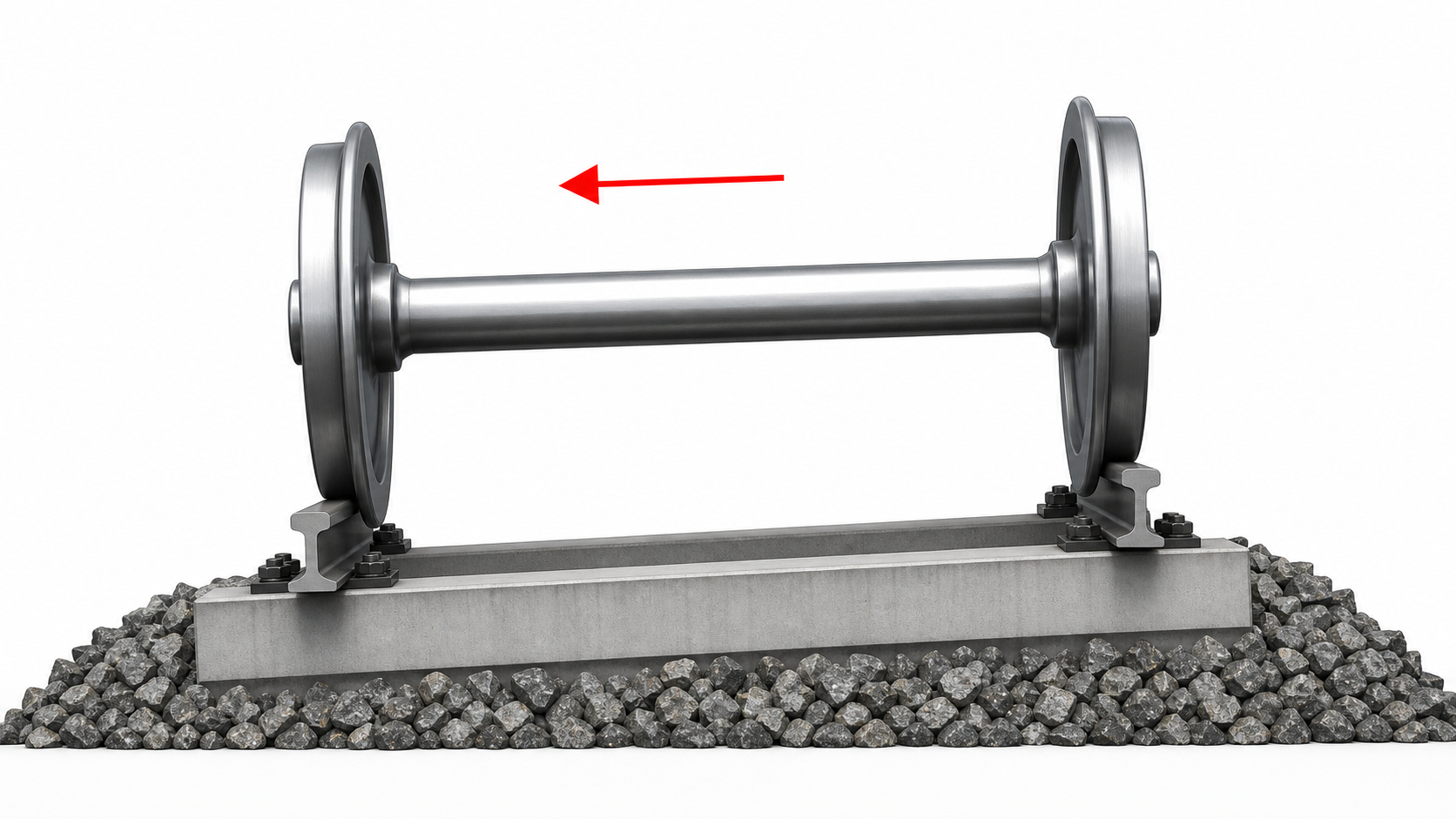
Excessive cant causes passengers to feel pushed towards the inside of the curve (inward lean) and can cause uneven loading of the rails, leading to head wear on the inner rail and potential track spreading or overturning in extreme cases. This is the opposite wheelset tendency from cant deficiency: the wheelset is biased toward the inner rail (Figure 5.8).

Figure 5.7 Cant excess: wheelset bias toward the inner rail.

Cant excess limits depend on whether the line is new, existing, mixed-traffic, or pure passenger traffic. As indicative Bane NOR technical regulation values:

• New mixed-traffic lines: normal requirement \(I_{e,\mathrm{max}} = 70\) mm, minimum requirement \(I_{e,\mathrm{max}} = 100\) mm.

• Existing conventional lines: \(I_{e,\mathrm{max}} = 90\) mm for \(R \leq 600\) m and \(I_{e,\mathrm{max}} = 110\) mm for \(R > 600\) m.

5.3.5 Applied Cant Limits

The applied cant \(h_m\) must satisfy both the cant deficiency and cant excess criteria for all trains using the line. For a mixed-traffic line with maximum speed \(v_\mathrm{max}\) and minimum speed \(v_\mathrm{min}\):

\[ h_\mathrm{th}(v_\mathrm{max}) - I_\mathrm{max} \;\leq\; h_m \;\leq\; h_\mathrm{th}(v_\mathrm{min}) + I_{e,\mathrm{max}}, \qquad h_m \leq h_{m,\mathrm{max}} \label{eq:applied_cant_bounds} \]

The lower bound ensures that the fastest trains (\(v_\mathrm{max}\)) experience at most \(I_\mathrm{max}\) of cant deficiency: \(h_m \geq h_\mathrm{th}(v_\mathrm{max}) - I_\mathrm{max}\). The upper bound ensures that the slowest trains (\(v_\mathrm{min}\)) experience at most \(I_{e,\mathrm{max}}\) of cant excess: \(h_m \leq h_\mathrm{th}(v_\mathrm{min}) + I_{e,\mathrm{max}}\).

This inequality is a compact way to see why mixed-traffic alignment design is difficult. A large cant improves the fast passenger-train case but worsens the slow freight-train or stopping-train case. If the lower bound exceeds the upper bound, the specified speed mix is not feasible with the chosen radius and limits; the designer must increase the radius, separate traffic, reduce the speed differential, or obtain a different vehicle approval basis.

For new lines in Norway:

• Maximum applied cant is normally 150 mm; pure passenger lines may permit higher values under the normal/minimum requirements stated in technical regulations.

• For \(v \leq 40\) km/h, cant should normally not be introduced; if special circumstances require cant, it is normally limited to 60 mm. At such low speeds, there is little centrifugal effect to balance the raised outer rail, so cant mainly creates cant excess for slow or stopped trains.

• In curves where trains often stop, such as near platforms or planned signal stops, lower cant values are preferred to limit cant excess.

A speed-independent low-speed derailment check must also be satisfied. For new lines and line relocations, Bane NOR technical regulations use:

\[ h_m \leq \frac{R - 100}{2} \quad [\text{mm}] \label{eq:cant_derailment_new} \]

For existing conventional lines, the corresponding technical regulation check is:

\[ h_m \leq \frac{R - 50}{1.5} \quad [\text{mm}] \label{eq:cant_derailment_existing} \]

The design logic for mixed traffic is therefore an envelope problem: the applied cant must be high enough for the fastest trains, but low enough that the slowest trains do not experience excessive cant excess. Additional local limits may apply along platforms and in switches and crossings.

5.3.6 Worked Example: Cant and Speed

Example 1: A curve has \(R = 1600\) m, \(s = 1500\) mm, \(h = 150\) mm, \(g = 10\) m/s\(^2\), \(j_{u,\mathrm{max}} = 0.85\) m/s\(^2\). Find the equilibrium speed and the maximum allowable speed.

Equilibrium speed:

\[ v_\mathrm{eq} = \sqrt{\frac{R \cdot g \cdot h}{s}} = \sqrt{\frac{1600 \times 10 \times 0.150}{1.5}} = \sqrt{1600} = 40\,\text{m/s} = 144\,\text{km/h} \]

Maximum allowable speed:

\[ \begin{aligned} v_\mathrm{max} &= \sqrt{\left(\frac{g \cdot h}{s} + j_{u,\mathrm{max}}\right) R} = \sqrt{\left(\frac{10 \times 0.150}{1.5} + 0.85\right) \times 1600} \\ &= \sqrt{2960} \approx 54.4\,\text{m/s} = 196\,\text{km/h} \end{aligned} \]

Example 2: Find the required curve radius for \(v = 240\) km/h, \(h = 100\) mm, \(s = 1500\) mm, \(j_{u,\mathrm{max}} = 0.85\) m/s\(^2\), \(g = 10\) m/s\(^2\):

\[ R = \frac{v^2}{\dfrac{g \cdot h}{s} + j_{u,\mathrm{max}}} = \frac{(240/3.6)^2}{\dfrac{10 \times 0.100}{1.5} + 0.85} = \frac{4444}{0.667 + 0.85} \approx 2930\,\text{m} \]

With \(h = 150\) mm the required radius is approximately 2402 m. A higher cant allows a smaller radius at the same speed, a crucial insight for minimising earthwork on high-speed lines.

5.4 Transition Curve Design

Transition curves provide the gradual change needed between tangent track and circular curves, especially where cant and cant deficiency must change smoothly.

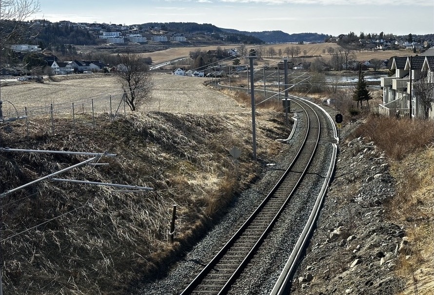
The photograph below shows a transition in its physical corridor. The curve, cant, overhead-line supports, and the surrounding land must be coordinated.

Electrified railway curve in Trondheim.

5.4.1 Purpose and Length Requirements

During the transition from straight to circular curve, the cant must be ramped up from zero to the full value \(h\). The transition must be long enough to satisfy three independent criteria simultaneously.

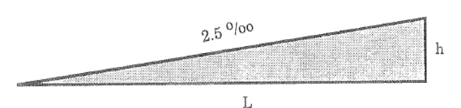
The three criteria below should be interpreted as serviceability and safety filters applied to the same geometric element. The cant-gradient criterion limits twist and wheel unloading, the rate of change of cant limits the roll input to the vehicle body, and the jerk criterion limits the rate at which passengers and vehicle suspensions experience uncompensated lateral acceleration. The final transition length is therefore the maximum of all applicable checks, rounded upward to a constructible value and coordinated with neighbouring alignment elements. The cant ramp in Figure 5.9 is a useful way to read the first check: a given cant height must be introduced over enough length to keep the gradient acceptable.

Figure 5.8 Cant ramp over a transition curve. The cant gradient relates the change in cant h to the transition length L_t and is one of the governing checks for transition design.

Criterion 1: Cant gradient \(\rho\) (derailment risk)

The cant gradient \(\rho\) is the change in cant per unit length along the transition:

\[ \rho = \frac{\Delta h}{\Delta L} \]

When \(\Delta h\) is inserted in millimetres and \(\Delta L\) in metres, \(\rho\) is obtained in mm/m, numerically equal to per mille:

\[ 1\,\mathrm{mm/m}=1\,‰. \]

A general maximum limit of \(\rho_\mathrm{max} \leq 2.5\,\mathrm{mm/m}=2.5\) ‰ (1:400) applies. Minimum transition length from this criterion:

\[ L_1 \geq \frac{h}{\rho_\mathrm{max}} \label{eq:L1} \]

Criterion 2: Rate of change of cant \(\Delta D\) (comfort)

The rate of change of cant with time is \(\Delta D = \Delta h / \Delta t = v \cdot \rho\). Typical limits are \(\Delta D_\mathrm{max} = 35\)–70 mm/s for new lines in Bane NOR technical regulations, with other values used for existing lines and approved rolling stock. Minimum transition length:

\[ L_2 \geq v \cdot \frac{h}{\Delta D_\mathrm{max}} \label{eq:L2} \]

Criterion 3: Rate of change of lateral acceleration \(\psi\) (jerk)

The rate of change of uncompensated lateral acceleration (jerk) is:

\[ \psi = \frac{\Delta j_u}{\Delta t} \]

Maximum permitted jerk is commonly expressed in railway standards as the rate of change of cant deficiency, \(\mathrm{d}I/\mathrm{d}t\). For new Bane NOR lines this corresponds to approximately \(\psi_\mathrm{max} = 0.33\)–\(0.46\) m/s\(^3\) under normal/minimum requirements, while existing lines and special rolling stock may use other values. The uncompensated lateral acceleration at maximum cant deficiency \(I_\mathrm{max}\) is \(j_{u,\mathrm{max}} = g\,I_\mathrm{max}/s\), where \(g \approx 9.81\) m/s\(^2\) and \(s \approx 1.5\) m is the effective track spacing between rolling-contact points. In this expression \(I_\mathrm{max}\) and \(s\) must use the same length unit. If \(I_\mathrm{max}\) and \(s\) are both inserted in millimetres, their ratio is dimensionless; if SI units are used, \(I_\mathrm{max}\) must first be converted to metres. Since \(I\) itself depends on speed, detailed technical regulation checks based on the rate of change of cant deficiency may require iteration. Minimum transition length from the jerk criterion:

\[ L_3 \geq v \cdot \frac{j_{u,\mathrm{max}}}{\psi_\mathrm{max}} = \frac{v\,g\,I_\mathrm{max}}{s\,\psi_\mathrm{max}} \label{eq:L3} \]

The governing minimum transition length is:

\[ L_{t,\mathrm{min}} = \max(L_1,\, L_2,\, L_3) \label{eq:Lt} \]

EN standards and national rules also specify additional absolute minimum requirements and checking equations [10, 88]. The exact set depends on the design case, but typical preliminary checks include those in Table 5.3.

Check	Input units	Interpretation
\(L > 4.5\) m	N/A	Absolute minimum length.
\(L > 0.41 V_\mathrm{max}\)	\(V_\mathrm{max}\) in km/h	Minimum length proportional to design speed.
\(L > 8 I_\mathrm{lim} v_\mathrm{max}\)	\(I_\mathrm{lim}\) in m; \(v_\mathrm{max}\) in m/s	Rate-of-change check using the larger relevant cant-deficiency or cant-excess limit.
\(L > 0.118 V^3/R\)	\(V\) in km/h; \(R\) in m	Curvature/speed check expressed in compact railway units.

Table 5.3 Additional transition-curve length checks. Project design must use the current standard and technical regulation case table.

5.4.2 Worked Example: Transition Curve Length

Example 3: Given \(v = 180\) km/h \(= 50\) m/s, \(h = 100\) mm, a stringent project limit \(\Delta D_\mathrm{max} = 28\) mm/s, \(\rho_\mathrm{max} = 2.5\) ‰, \(j_{u,\mathrm{max}} = 0.65\) m/s\(^2\), \(\psi_\mathrm{max} = 0.16\) m/s\(^3\).

\[ L_1 \geq \frac{100}{2.5} = 40\,\text{m} \]

\[ L_2 \geq 50 \times \frac{100}{28} = 178.6\,\text{m} \]

\[ L_3 \geq 50 \times \frac{0.65}{0.16} = 203.1\,\text{m} \]

The jerk criterion governs; \(L_{t,\mathrm{min}} = 203.1\) m \(\approx 205\) m (rounded up to the next 5 m).

Example 4: Transition length when \(j_u\) is not given. Consider a curve with \(R=1000\) m, \(v=90\) km/h \(=25\) m/s, applied cant \(h=60\) mm, \(\Delta D_\mathrm{max}=28\) mm/s, \(\rho_\mathrm{max}=2.5\) ‰, \(\psi_\mathrm{max}=0.16\) m/s\(^3\), \(s=1500\) mm, and \(g=9.81\) m/s\(^2\). Here the uncompensated lateral acceleration is not supplied directly, so it must first be calculated from the curve geometry and speed.

\[ L_1 \geq \frac{60}{2.5} = 24\,\text{m} \]

\[ L_2 \geq 25 \times \frac{60}{28} = 53.6\,\text{m} \]

First calculate the uncompensated lateral acceleration:

\[ j_u = \frac{v^2}{R} - \frac{gh}{s} = \frac{25^2}{1000} - \frac{9.81 \times 60}{1500} = 0.233\,\text{m/s}^2 \]

where \(h\) and \(s\) are both inserted in millimetres in the second term, so their ratio is dimensionless. The jerk criterion then gives

\[ L_3 \geq \frac{vj_u}{\psi_\mathrm{max}} = \frac{25 \times 0.233}{0.16} = 36.4\,\text{m} \]

The rate-of-change-of-cant criterion governs, so the minimum transition length is \(L_{t,\mathrm{min}} = 53.6\) m. In a design submission this value should be rounded upward and checked against the absolute minimum transition-length requirements in Table 5.3.

5.5 Vertical Alignment

Vertical alignment controls gradients and vertical curves, and must be coordinated with the horizontal alignment to avoid operational and comfort problems.

5.5.1 Vertical Gradient

The vertical gradient (stigning/fall, expressed in per mille (‰) or percent) describes the slope of the track in the vertical plane. A positive gradient indicates an ascent; a negative gradient a descent. In the longitudinal profile, this slope is read from the rise over a defined horizontal run (Figure 5.10). For a horizontal distance \(L\) and elevation difference \(\Delta H\), the signed gradient is \(c_+ = +1000\,\Delta H/L\,[‰]\) for an ascent and \(c_- = -1000\,\Delta H/L\,[‰]\) for a descent.

Figure 5.9 Vertical-gradient sign convention and 1000 m determining chord.

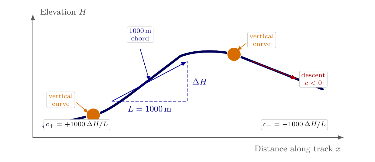
The determining gradient is defined as the steepest average gradient found by connecting any two points 1000 m apart along the longitudinal profile [124, 141]. This definition is significant for Norwegian mountain lines where the gradients over long distances are the binding design constraint, rather than the maximum gradient at any single point.

5.5.2 Vertical Curves

Vertical curves connect two straight gradient lines so that the change in vertical acceleration is gradual. Without a vertical curve, the instantaneous change in gradient at a grade break would produce unacceptable dynamic forces and passenger discomfort. Railway vertical curves are commonly represented by large-radius circular arcs in Norwegian design rules, while parabolic curves are also widely used in international railway and road practice because they give a constant rate of change of gradient.

For a grade change from \(c_1\) to \(c_2\), where gradients are expressed in decimal form, the change in gradient is:

\[ \Delta c = |c_2 - c_1| \label{eq:vertical_gradient_change} \]

For a circular vertical curve with radius \(R_v\), the tangent length on each side of the point of vertical intersection is denoted \(l\) in the construction figure from Bane NOR's sporgeometri material [18]. For small railway gradients it is approximately:

\[ l = \frac{R_v \Delta c}{2} \label{eq:vertical_tangent_length} \]

and the total vertical-curve length is:

\[ L_v = R_v \Delta c = 2l \label{eq:vertical_curve_length} \]

The construction behind this relationship is the same for low-point and high-point grade changes (Figure 5.11).

Figure 5.10 Vertical-curve construction for low-point and high-point grade changes. Source: Bane NOR track-geometry material [18].

Requirement	Design formula	Absolute lower radius
Normal design radius	\(R_{v,\mathrm{normal}} = V^2/2.6\)	About 4000 m
Minimum design radius	\(R_{v,\mathrm{min}} = V^2/3.9\)	About 2500 m

Table 5.4 Bane NOR vertical-curve radius requirements for new lines and line relocations [10]. Use $V$ in km/h and $R_v$ in metres.

Existing lines, switches and crossings, platform areas, and special structures must be checked against the current Technical Regulations case table for the actual design case.

5.5.3 Worked Example: Vertical Gradient and Vertical Alignment

The following example combines vertical-gradient calculation, vertical-curve sizing, and a geometry-overlap check. The point of vertical intersection (PVI) is where the incoming and outgoing straight gradient lines meet before they are connected by a vertical curve. It is located at km 25+000. The elevation rises from 112.00 m at km 24+000 to 120.00 m at the PVI, and then falls to 116.00 m at km 26+000. The design speed is 160 km/h, and a horizontal transition begins 50 m before the PVI. Determine the signed gradients, the normal and minimum vertical-curve radii, the associated curve lengths, and whether the horizontal transition satisfies the 15 m separation rule.

The signed gradients are

\[ \begin{aligned} c_1&=+1000\frac{120.00-112.00}{1000}\\ &=+8\,‰,\\ c_2&=+1000\frac{116.00-120.00}{1000}\\ &=-4\,‰. \end{aligned} \]

Before using the vertical-curve equations, convert the gradients from per mille to decimal form: \(c_1=+0.008\) and \(c_2=-0.004\). Thus,

\[ \Delta c=|0.008-(-0.004)|=0.012. \]

At 160 km/h, the resulting normal and minimum design radii are

\[ R_{v,\mathrm{normal}}=\frac{160^2}{2.6}=9846\,\mathrm{m}, \qquad R_{v,\mathrm{min}}=\frac{160^2}{3.9}=6564\,\mathrm{m}. \]

Both values exceed the corresponding absolute lower-radius floors in Table 5.4.

For the normal radius,

\[ l_{\mathrm{normal}}=\frac{9846\times0.012}{2}=59.1\,\mathrm{m}, \qquad L_{v,\mathrm{normal}}=118.2\,\mathrm{m}. \]

For the minimum radius,

\[ l_{\mathrm{min}}=\frac{6564\times0.012}{2}=39.4\,\mathrm{m}, \qquad L_{v,\mathrm{min}}=78.8\,\mathrm{m}. \]

The horizontal transition begins at km 24+950. The normal-radius vertical curve begins at km \(25+000-59.1=24+940.9\), leaving only 9.1 m between the two boundaries. The minimum-radius curve begins at km \(25+000-39.4=24+960.6\), giving a boundary separation of 10.6 m. Both are below 15 m. The overlap therefore fails the normal separation rule and must be relocated or assessed as a combined three-dimensional vehicle–track problem.

5.5.4 Coordination of Horizontal and Vertical Geometry

Horizontal transition curves and vertical curves should be coordinated carefully. Combining a large change in curvature, cant, and vertical acceleration at the same location can increase wheel unloading and reduce passenger comfort. As a design principle, avoid placing the beginning or end of a horizontal transition curve at the same chainage as a vertical grade break. Bane NOR's Technical Regulations also restrict the coincidence of vertical curves with small radii (\(R_v < 10000\) m) and horizontal transition curves or turnouts; a separation of at least 15 m is normally required except in low-speed cases. If unavoidable, the geometry should be checked as a combined three-dimensional vehicle–track problem rather than as independent horizontal and vertical elements.

5.6 Chapter Summary

Train path. The alignment is the three-dimensional path that the vehicle must follow, and it therefore controls speed, comfort, lateral force, wear, construction feasibility and maintenance demand. Straight track, circular curves, transition curves, vertical gradients and vertical curves are not separate drafting elements; they combine to shape the dynamic environment experienced by vehicles and passengers.

Curves and cant. For a given curve radius, higher speed requires higher equilibrium cant. In practice, applied cant is limited by construction, maintenance and mixed-traffic operation, so some trains operate with cant deficiency and others with cant excess. The design task is to choose a combination that keeps passenger comfort, wheel–rail forces and freight operation within acceptable limits rather than optimising for only one train type.

Transitions. A transition curve gradually introduces curvature and cant, reducing lateral jerk and avoiding abrupt changes in wheel–rail force. Its length must be sufficient for cant ramp, curvature change and comfort requirements. Short transitions may satisfy a simple geometric connection, but they can produce poor ride quality, increased maintenance and speed restrictions, especially on high-speed or mixed-traffic lines.

Vertical geometry. Gradients influence train resistance and braking requirements, while vertical curves control comfort and the rate of change in vertical acceleration. Horizontal and vertical geometry must also be coordinated so that curves, transitions, bridges, tunnels, platforms and drainage constraints do not create conflicting requirements. A geometrically valid line is not necessarily operationally good if the vertical and horizontal elements are poorly combined.

Design compromise. Standards provide limits for cant, cant deficiency, transition length, gradients and vertical curves, but the engineer must still judge how the railway will be used. Passenger speed, freight speed, stopping pattern, terrain, constructability, future maintenance and possible tilting trains all influence the final geometry. The best design is one where speed, comfort, safety and maintainability support one another.

Assignments

Assignment 1: High-speed alignment and transition design

A new high-speed railway line is designed for \(v_\mathrm{max} = 250\) km/h. The alignment must negotiate a direction change of 15\(^\circ\) in difficult terrain.

(a) Before calculating, identify two possible alignment strategies for passing through the terrain (for example a tighter surface route, a longer tunnel, or a longer detour). State the main benefit and drawback of each.

(b) Explain why forecast traffic volume, construction cost, and future maintenance cost must be considered before choosing the final route.

(c) Determine the minimum curve radius required if \(h = 150\) mm and \(I_\mathrm{max} = 100\) mm.

(d) Determine the minimum transition curve length using \(I_\mathrm{max}=100\) mm, \(\rho_\mathrm{max} = 2.5\) ‰, \(\Delta D_\mathrm{max} = 28\) mm/s, and \(\psi_\mathrm{max} = 0.16\) m/s\(^3\). Which criterion governs?

(e) Recommend a preferred strategy for this location, explaining what extra information you would request before freezing the alignment.

Assignment 2: Mixed-traffic cant design

A line carries both high-speed passenger trains (\(v = 200\) km/h) and freight trains (\(v_\mathrm{min} = 60\) km/h). For a curve with \(R = 2000\) m, determine:

(a) The theoretical cant for the passenger trains

(b) The theoretical cant for the freight trains

(c) The range of permissible applied cant \(h_m\) satisfying both cant deficiency (\(I_\mathrm{max} = 100\) mm) and cant excess (\(I_{e,\mathrm{max}} = 100\) mm) requirements

(d) The recommended applied cant for mixed traffic

Line parameters: \(R = 2000\) m, \(v_\mathrm{fast} = 200\) km/h, \(v_\mathrm{slow} = 60\) km/h.

Assignment 3: Tilting train curve speed

A tilting train with active tilting (\(\alpha_T = 6^\circ\), equivalent \(h_t = s \cdot \tan\alpha_T \approx 157\) mm) operates on a curve with \(R = 800\) m and track cant \(h = 120\) mm. Calculate the maximum speed achievable by the tilting train if the permitted passenger-perceived cant deficiency is \(I_\mathrm{p} = 100\) mm. Then discuss why the resulting speed must still be checked against vehicle approval, track-force, and Bane NOR technical regulation limits for the actual rolling stock.

Assignment 4: Multi-curve speed optimisation

An existing section consists of three curves in sequence. The sign of the radius indicates curve direction; use the absolute radius for speed calculations. The maximum permitted cant deficiency is \(I_\mathrm{max}=100\) mm.

Curve	\(R\) (m)	\(L_t\) (m)	\(h\) (mm)
1	\(-1485\)	240	100
2	2150	276	100
3	2400	300	30

Use \(\rho_\mathrm{max}=2.5\) ‰, \(\Delta D_\mathrm{max}=35\) mm/s, and \(\psi_\mathrm{max}=0.33\) m/s\(^3\). For the transition jerk check, use \(j_{u,\mathrm{max}}=0.85\) m/s\(^2\) as the project comfort limit.

(a) Calculate the maximum speed for each curve and identify the governing speed for the whole section.

(b) Check whether the provided transition lengths are sufficient at the curve-specific maximum speeds.

(c) The cant may be increased, but not above 150 mm. Propose cant changes that maximise the speed of the whole section, and recheck the critical transition lengths.

(d) Explain why the maximum calculated speed is not automatically the operational speed that should be published for the section.

Assignment 5: Single-curve transition check

A single curve has the following geometry:

Parameter	Value
Effective track spacing	\(s = 1500\) mm
Radius	\(R = 1200\) m
Transition length	\(L_t = 100\) m
Applied cant	\(h = 150\) mm
Maximum cant deficiency	\(I_\mathrm{max} = 100\) mm
Maximum cant excess	\(I_{e,\mathrm{max}} = 70\) mm
Cant-gradient limit	\(\rho_\mathrm{max}=2.5\) ‰
Rate-of-change-of-cant limit	\(\Delta D_\mathrm{max}=35\) mm/s
Jerk limit	\(\psi_\mathrm{max}=0.33\) m/s\(^3\) with \(j_{u,\mathrm{max}}=0.85\) m/s\(^2\)

(a) Calculate the maximum speed from the circular-curve cant-deficiency check.

(b) Check the transition length at that speed. If the transition is too short, calculate the transition-limited speed and identify the governing criterion.

(c) If the applied cant is reduced to \(h=130\) mm for slow mixed traffic, calculate the minimum speed required by the cant-excess limit.

(d) Comment on whether this is a robust mixed-traffic design and suggest one geometry change that would improve it.

Assignment 6: Vertical curve and geometry overlap

A gradient profile has an ascending grade of \(+8\) ‰ meeting a descending grade of \(-4\) ‰ at a crest. The design speed at this location is 160 km/h.

(a) Determine the normal and minimum required vertical curve radii.

(b) Calculate the tangent length \(l\) on each side of the grade break.

(c) A transition curve for a horizontal curve starts 50 m before the grade break. Explain why this is problematic and how it should be resolved.