Wheel–Rail Interaction
When a railway vehicle moves along a track, all support, guidance, traction and braking forces pass through a small contact patch between steel wheel and steel rail. This chapter therefore treats the wheel–rail interface itself: how wheel and rail profiles guide the vehicle, how the contact patch is calculated, and how excessive lateral-to-vertical force can lead to flange climbing.
Chapter 1 covers traffic loading and preliminary track-stress checks, and Chapter 7 covers the broader train–track dynamic system. Those topics are used only as background here. The emphasis in the present chapter is local wheel–rail interaction: rolling-radius difference, equivalent conicity, curve negotiation, straight track hunting, Hertzian contact, and derailment criteria.
8.1 Introduction
The wheel–rail interface is small, but it controls several large-scale behaviours:
-
Guidance: the rolling-radius difference between the two wheels steers the wheelset in curves and recentres it on tangent track.
-
Contact: the normal load is carried over a small elastic patch, often only a few square centimetres, producing high contact pressures.
-
Friction and creepage: tangential forces arise when the wheel and rail have small relative slip in the longitudinal, lateral or spin direction.
-
Derailment safety: a combination of high lateral force, low vertical force and unfavourable contact angle can lead to flange climbing.
Dynamic train movement, track receptance and vertical load amplification are treated in Chapter 7. In this chapter they are mentioned only when they affect the local wheel–rail force ratio or contact condition.
8.2 Wheelsets, Wheel Profiles and Conicity
Wheel–rail guidance starts with the wheelset itself. A railway wheel is not a cylindrical roller: its tread is shaped, the rail is inclined, and the two wheels are rigidly connected by an axle. These basic geometric details explain why a wheelset can steer in curves, why it oscillates on straight track, and why equivalent conicity is one of the central profile quantities in vehicle–track interaction.
8.2.1 The Wheelset
A wheelset consists of two wheels rigidly coupled by an axle. This rigid coupling is the fundamental feature that distinguishes a railway wheelset from a road-vehicle axle with independently rotating wheels. Both railway wheels have the same angular velocity. If the left and right rolling radii differ, the two wheels try to roll different distances per revolution, and the wheelset must yaw.
The wheelset serves three principal functions:
-
It provides the necessary clearance between the vehicle body and the track structure.
-
It provides guidance, keeping the vehicle on the correct path.
-
It transmits traction and braking forces to the rails.
The design details of a wheelset, such as brake discs, journals and gearboxes, depend on vehicle type. For wheel–rail guidance, however, the decisive point is the rigid axle and the profile-dependent rolling-radius difference. Before reducing the geometry to a single conicity value, the actual wheel profile must therefore be identified.
8.2.2 Wheel Profiles
A wheel profile is the cross-section of the wheel tread and flange. It is a geometric definition of the running surface, not merely a sketch of a wheel. The running tread carries the normal rolling contact on tangent track and large-radius curves. The flange root and flange provide additional lateral guidance when tread steering is not sufficient, for example in tight curves or under unfavourable contact conditions.
Real wheel profiles are not perfect cones. They are built from straight parts, arcs, fillets and flange geometry so that contact can migrate gradually across the tread as the wheelset moves laterally. In European practice, standardized tread profiles are specified in EN 13715, and a common example is the UIC/ORE S1002 worn-type profile, which was introduced as a profile adapted to wear [90, 112, 113]. Figure 8.1 shows this important point: the nominal tread slope is only one part of a much richer profile geometry.
![UIC/ORE S1002 wheel profile [112].](../../assets/chapters/ch08/original/figures_lecture_crops/fig_s1002_wheel_profile_lecture_crop.png)
The rail profile and rail inclination must be considered together with the wheel profile. A wheel profile that gives favourable contact on one rail profile may give a different contact-point path and a different rolling-radius difference on another rail. This is why the next subsection first defines the simple conicity concept and then introduces equivalent conicity as a wheel–rail profile-pair quantity.
8.2.3 Wheel Conicity
The wheel tread is not cylindrical but slightly cone-shaped. This taper gives the wheelset its self-steering ability. Figure 8.2 defines the basic conicity measure.
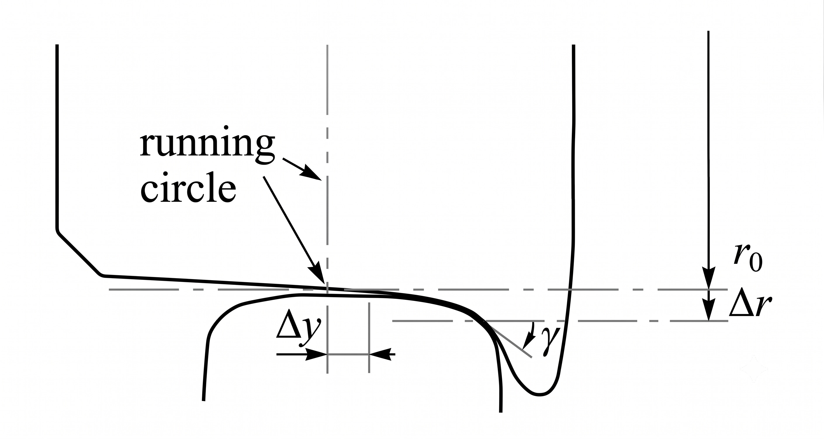
Let \(\delta r\) denote the change in rolling radius of one wheel from the centred position, and let \(y\) denote the lateral displacement of the wheelset. The conicity \(\lambda\) is defined as
Typical values for nominal tread conicity are 1:20 (\(\lambda = 0.05\)) or 1:40 (\(\lambda = 0.025\)). Real wheels and rails are not perfect cones. The practical quantity is therefore the equivalent conicity \(\lambda_{eq}\), which is obtained from the actual wheel and rail profiles over a specified lateral displacement range.
For a wheelset displaced laterally by \(y\) from the centred position, a linearised equivalent-conicity model writes the left and right rolling radii as
where \(r_0\) is the nominal rolling radius. The total rolling-radius difference between the two wheels is therefore
Equivalently, \(\lambda_{eq}=\Delta r/(2y)\) for the chosen lateral displacement range.
Rail inclination also matters. Rails are normally inclined inward, for example 1:20 or 1:40, so the rail-head normal better matches the wheel-tread normal in ordinary tread contact. As the wheelset shifts sideways, the contact points move on both profiles. The local wheel slope, rail inclination and rail-head curvature together determine the contact angle, the rolling-radius difference and the equivalent conicity. This is why a constant conicity model is useful for derivations, but profile measurements are needed for real vehicles.
8.3 Wheel–Rail Guidance in Curves
Curve guidance is the first place where the rolling-radius difference becomes a practical steering mechanism. The outer wheel must travel a longer path than the inner wheel. A coned wheelset can do this without axle slip if it shifts laterally so that the outer wheel runs on a larger rolling radius and the inner wheel runs on a smaller rolling radius, as shown in Figure 8.3.
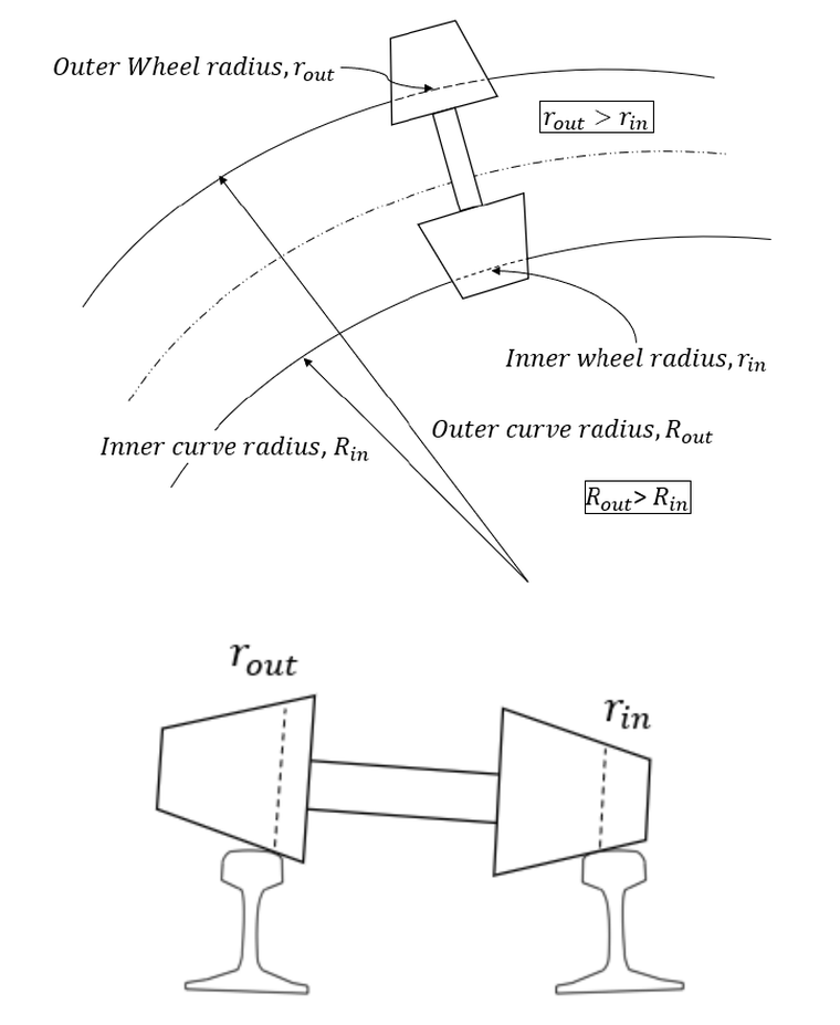
The derivation below is an ideal geometric model. It assumes straight coned wheels, constant conicity, no flange contact, pure rolling at the contacts, constant speed, no inertia forces, balanced-speed curving and a free wheelset not constrained by a bogie suspension. These assumptions isolate the basic guidance mechanism. Real vehicles depart from the model through suspension stiffness, creep forces, profile wear, flange contact and unbalanced lateral acceleration.
Consider a wheelset negotiating a curve of radius \(R\). The outer wheel rolls on path radius
and the inner wheel rolls on path radius
where \(b_0\) is half the effective spacing between the two rolling-contact points.
For radially perfect steering (no sliding), the ratio of rolling circumferences must equal the ratio of path radii:
Let the wheelset have nominal rolling radius \(r_0\). If the wheelset shifts laterally, the outer and inner rolling radii can be written as
where \(\delta r\) is the per-wheel rolling-radius change from the centred position. Substituting Equation 8.5 into Equation 8.4 gives
After rearrangement,
or equivalently
Since the conicity relation is \(\delta r=\lambda_{eq}y\), the lateral displacement needed for radial steering is
For example, with \(r_0 = 0.5\) m, equivalent conicity 1:20 (\(\lambda_{eq} = 0.05\)), \(b_0 = 0.75\) m and \(R = 500\) m, the required lateral displacement is
The wheelset must therefore shift about 15 mm outward to steer perfectly through this curve. If the available tread clearance is smaller than this, the wheelset cannot remain in pure tread contact and flange contact becomes likely.
For real curving, this ideal result is a reference rather than a guarantee. A bogie wheelset has yaw stiffness, primary suspension, creepage and limited clearance. In tight curves, or with worn wheel and rail profiles, the leading wheelset develops an angle of attack and the outer-wheel flange contacts the gauge corner of the high rail. The contact normal is then no longer close to vertical: it is inclined by the local flange and rail-gauge-face geometry, so part of the normal force contributes directly to lateral guidance. This is why curve negotiation links rolling-radius difference, equivalent conicity, rail inclination, flange contact, wear, squeal noise and derailment sensitivity.
8.4 Wheel–Rail Guidance on Straight Track
On straight track there is no curve radius to follow, but the same coned-wheel geometry still acts whenever the wheelset is displaced laterally. The result is a sinusoidal motion of the free wheelset. In a real vehicle, suspension, damping, creepage and profile wear decide whether this motion decays or develops into hunting.
8.4.1 Klingel's Formula
The classical sinusoidal motion of a free coned wheelset is known as Klingel hunting. The derivation below follows the geometry in Figure 8.4: the lateral displacement, yaw angle and unequal rolling velocities are the quantities that produce the sinusoidal path. The derivation is purely kinematic: it assumes pure rolling, constant speed, small angles, a rigid wheelset, no suspension and no creep-force limit.
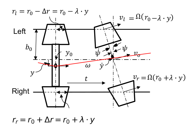
Let \(\psi\) be the yaw angle of the wheelset and let \(x\) be distance along the track. For small angles,
The rolling-radius difference in Equation 8.3 makes one wheel roll farther than the other. The corresponding curvature of the wheelset path is
Combining Equations 8.10 and 8.11 gives
The solution is sinusoidal:
with the Klingel wavelength
At running speed \(v\), the corresponding kinematic hunting frequency is
when \(v\) is expressed in m/s. Equations 8.2–8.15 are often the most useful Klingel formula family: rolling radii, radius difference, spatial wavelength and temporal frequency.
The main point of the formula is the square-root dependence on equivalent conicity: for a fixed wheel radius and contact spacing, lower \(\lambda_{eq}\) gives a longer wavelength, while higher \(\lambda_{eq}\) gives a shorter wavelength. The wavelength is the distance over one full sinusoidal wheelset cycle, marked as \(L\) in Figure 8.5; it is a kinematic path length, not a separate vehicle vibration mode.
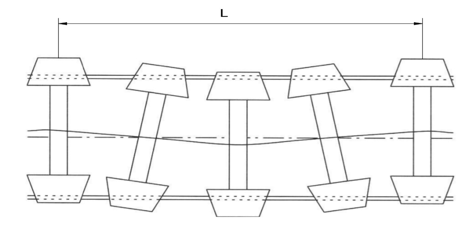
Example.
For \(b_0 = 0.75\) m, \(r_0 = 0.5\) m and \(\lambda_{eq}=1/20\):
If the same wheelset runs at 160 km/h, \(v=44.4\) m/s and \(f_K = 44.4/17 \approx 2.6\) Hz.
8.4.2 Hunting Stability and Limit Cycles
The Klingel wavelength describes the natural kinematic path of a free coned wheelset. Real vehicles also have suspension stiffness, damping, inertia, creep forces and wheel– rail friction. These effects decide whether a lateral disturbance decays, remains as a bounded oscillation or grows into unstable hunting.
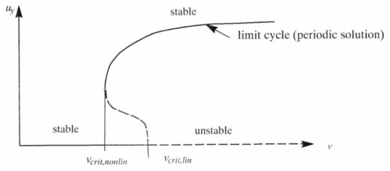
The nonlinear hunting-stability picture is usually shown as a speed–amplitude diagram. The horizontal axis is vehicle speed \(v\), while the vertical axis represents the lateral oscillation amplitude. The two important speeds are the nonlinear critical speed \(v_{\mathrm{crit,nonlin}}\) and the linear critical speed \(v_{\mathrm{crit,lin}}\), as indicated in Figure 8.6.
Below the nonlinear critical speed.
For \(v < v_{\mathrm{crit,nonlin}}\), the vehicle is stable for the relevant disturbance amplitudes. A lateral excitation may start a hunting-like oscillation, but suspension damping and wheel–rail creep forces remove energy from the motion, so the oscillation decays and the wheelset returns toward the centred running position.
Between the nonlinear and linear critical speeds.
For \(v_{\mathrm{crit,nonlin}} < v < v_{\mathrm{crit,lin}}\), the vehicle is conditionally stable. Small disturbances still decay, but a sufficiently large disturbance can cross the unstable boundary in the diagram. The motion then does not grow without limit; instead it approaches a finite periodic oscillation, called the limit cycle. This is why a vehicle can pass a small-disturbance stability check and still be sensitive to large lateral inputs from track irregularities, impacts or profile changes.
Above the linear critical speed.
For \(v > v_{\mathrm{crit,lin}}\), the centred running state is linearly unstable. Even small disturbances tend to grow until nonlinear effects, flange contact, suspension limits or wheel–rail friction restrict the amplitude. Operation in this range is therefore associated with self-excited hunting and is not acceptable for stable service.
8.4.3 Limitations of the Simple Conicity Model
The kinematic conicity model makes strong simplifying assumptions:
-
Pure rolling (no creep) and constant speed.
-
No track irregularity.
-
Constant, linearised conicity.
-
No bogie suspension or inertia.
In practice, wheel and rail profiles are complex curves whose equivalent conicity varies with lateral displacement [116, 98]. The same wheel profile can therefore behave differently on different rail profiles or rail inclinations. A low equivalent conicity improves high-speed hunting stability, but it may give insufficient rolling-radius difference in tight curves. A high equivalent conicity improves steering in curves, but it shortens the Klingel wavelength and reduces the hunting-stability margin.
8.5 Wheel–Rail Contact Mechanics
The small contact patch between wheel and rail carries very large normal and tangential forces. Contact mechanics is therefore central to guidance, wear, rolling contact fatigue and flange-climbing derailment. The same contact conditions later explain rail-head wear and RCF defects in Chapter 15, and rolling-noise excitation in Chapter 10.
8.5.1 Contact Regions
Three geometric contact regions can be distinguished (Figure 8.7):
- Region A: Tread to rail head
-
The most common contact situation on tangent track. The contact area is relatively large and contact stresses are moderate.
- Region B: Flange to gauge corner
-
Occurs in tight curves when the leading wheelset usually presses the outer wheel flange against the gauge face of the high rail. The contact area is much smaller, leading to very high contact stresses and rapid wear on both the flange and the gauge corner of the rail.
- Region C: Field-side contact
-
The least likely situation, with intermediate contact area but undesirable lateral force direction.
![Three wheel–rail contact regions (A, B, C) distinguished by location and stress level [113].](../../assets/chapters/ch08/original/figures_lecture_crops/fig_contact_regions_lecture_enhanced.png)
Contact can be further classified as conformal (larger contact area, e.g. worn flange/gauge corner) or non-conformal (small contact area, standard tread–head contact).
8.5.2 Normal and Tangential Contact
The normal contact force \(N\) is mainly governed by wheel load and contact geometry. The tangential forces are governed by small relative motions between wheel and rail:
-
Longitudinal creepage: caused by traction, braking or a small mismatch between rolling speed and vehicle speed.
-
Lateral creepage: caused by lateral motion and angle of attack.
-
Spin creepage: caused by relative rotation of the contact patch about the normal direction.
For small creepages, tangential force is approximately proportional to creepage. At higher creepage the force saturates at the friction limit:
where \(X\) is longitudinal creep force, \(Y\) is lateral creep force and \(\mu\) is the wheel–rail coefficient of friction. Curving, hunting and flange climbing are therefore not only geometric problems: they depend on whether the contact patch can provide the required tangential force without sliding.
8.5.3 Hertzian Contact Theory
For non-conformal contact, Hertzian theory [113, 104] predicts an elliptical contact patch, provided the following assumptions hold:
-
Deformations and strains are small (linear elastic material).
-
The contact patch is small compared with the dimensions of both bodies (half-space assumption).
-
The surface curvatures near the contact are constant.
-
The surfaces are smooth and frictionless.
-
Only elastic displacements occur.
-
Both bodies are homogeneous and isotropic.
Figure 8.8 identifies the wheel and rail radii used in the Hertz contact calculation.
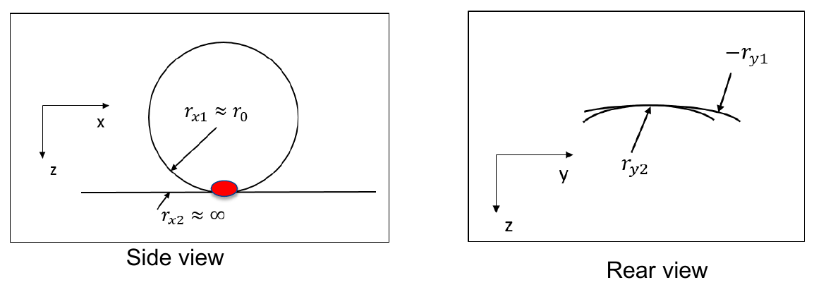
The geometry is described by four principal radii of curvature:
Two auxiliary parameters \(A\) and \(B\) are defined:
and the Hertz angle:
The constants \(m\) and \(n\) in the semi-axis equations are not material constants. They are geometric Hertz constants read from Table 8.1 using the Hertz angle \(\theta\). If \(\theta\) lies between two tabulated values, use linear interpolation. For example, \(\theta=130^\circ\) gives \(m=0.641\) and \(n=1.754\), while \(\theta=123.4^\circ\) is obtained by interpolating between \(120^\circ\) and \(125^\circ\). For lookup, read each three-column block from top to bottom, moving from the left block to the centre and then the right; \(\theta\) increases throughout.
| \(\theta\) [\(^\circ\)] | \(m\) | \(n\) | \(\theta\) [\(^\circ\)] | \(m\) | \(n\) | \(\theta\) [\(^\circ\)] | \(m\) | \(n\) |
|---|---|---|---|---|---|---|---|---|
| 0.5 | 61.400 | 0.1018 | 55.0 | 1.611 | 0.678 | 130.0 | 0.6410 | 1.754 |
| 1.0 | 36.890 | 0.1314 | 60.0 | 1.486 | 0.717 | 135.0 | 0.6040 | 1.926 |
| 1.5 | 27.480 | 0.1522 | 65.0 | 1.378 | 0.759 | 140.0 | 0.5670 | 2.136 |
| 2.0 | 22.260 | 0.1691 | 70.0 | 1.284 | 0.802 | 145.0 | 0.5300 | 2.397 |
| 3.0 | 16.500 | 0.1964 | 75.0 | 1.202 | 0.846 | 150.0 | 0.4930 | 2.731 |
| 4.0 | 13.310 | 0.2188 | 80.0 | 1.128 | 0.893 | 160.0 | 0.4123 | 3.813 |
| 6.0 | 9.790 | 0.2552 | 85.0 | 1.061 | 0.944 | 170.0 | 0.3112 | 6.604 |
| 8.0 | 7.860 | 0.2850 | 90.0 | 1.000 | 1.000 | 172.0 | 0.2850 | 7.860 |
| 10.0 | 6.604 | 0.3112 | 95.0 | 0.944 | 1.061 | 174.0 | 0.2552 | 9.790 |
| 20.0 | 3.813 | 0.4123 | 100.0 | 0.893 | 1.128 | 176.0 | 0.2188 | 13.310 |
| 30.0 | 2.731 | 0.4930 | 105.0 | 0.846 | 1.202 | 177.0 | 0.1964 | 16.500 |
| 35.0 | 2.397 | 0.5300 | 110.0 | 0.802 | 1.284 | 178.0 | 0.1691 | 22.260 |
| 40.0 | 2.136 | 0.5670 | 115.0 | 0.759 | 1.378 | 178.5 | 0.1522 | 27.480 |
| 45.0 | 1.926 | 0.6040 | 120.0 | 0.717 | 1.486 | 179.0 | 0.1314 | 36.890 |
| 50.0 | 1.754 | 0.6410 | 125.0 | 0.678 | 1.611 | 179.5 | 0.1018 | 61.400 |
The combined elastic modulus is:
The semi-axes of the elliptical contact patch are:
where \(N\) is the normal contact force, \(a\) is the longitudinal semi-axis, and \(b\) is the lateral semi-axis of the elliptical contact patch.
The calculation can therefore be read as a chain from contact geometry to contact pressure: the radii determine \(A\) and \(B\), then the angle \(\theta\), the constants \(m\) and \(n\), the semi-axes \(a\) and \(b\), the area \(A_c\), and finally \(P_{z,\max}\). Figure 8.9 shows the two physical quantities behind the final pressure equations: the contact ellipse and the pressure distribution over it.
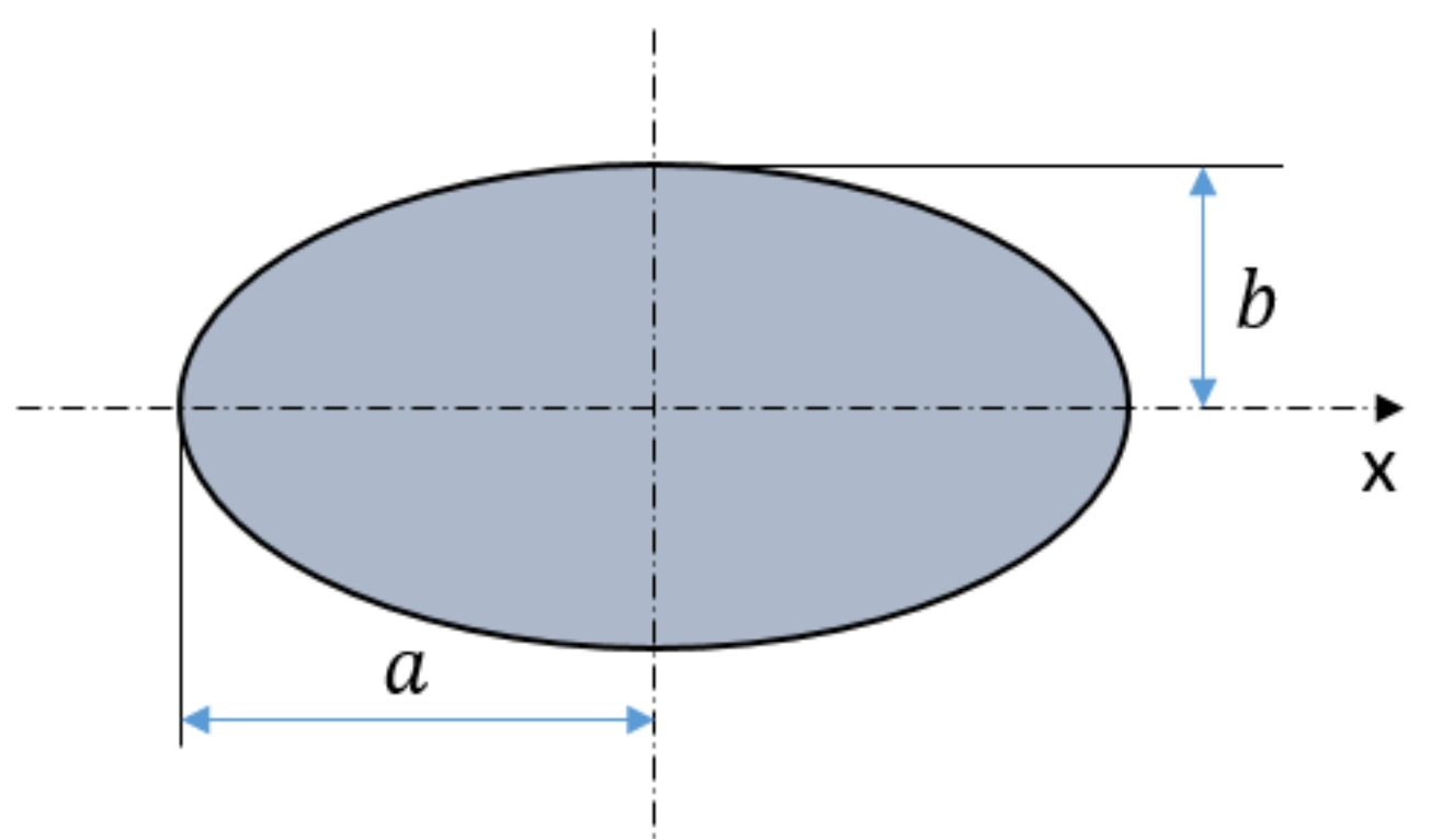
(a) Elliptical contact patch with semi-axes a and b.
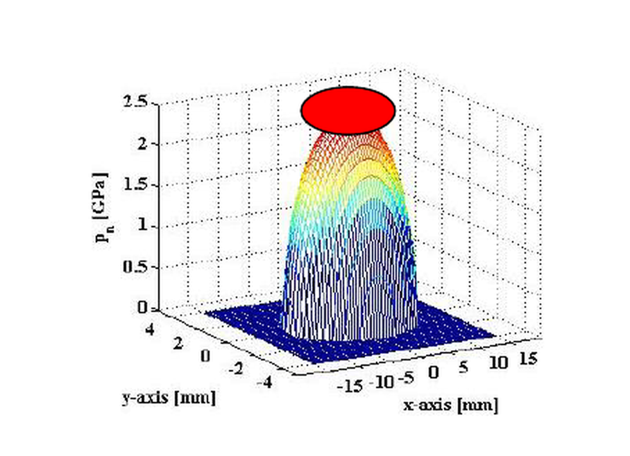
(b) Hertzian pressure distribution over the same contact patch.
The contact area and pressure distribution are:
The maximum contact pressure (at the centre of the patch) is:
Worked example (Hertzian contact patch).
With \(r_{x1} = 0.46\) m, \(r_{y1} = r_{y2} = 0.30\) m, \(r_{x2} \to \infty\), \(E = 210\,\text{GPa}\), \(\nu = 0.25\), and \(N = 60\) kN:
The corresponding mean Hertz pressure is
and the maximum pressure for the semi-ellipsoidal Hertz distribution is
This single example illustrates the calculation chain from geometry and load to contact ellipse size and pressure level. Changes in wheel radius, rail-head radius or wheel profile curvature are handled by repeating the same steps with the updated radii.
Simplified contact-stress estimate.
For quick checks, Eisenmann proposed a simplified formula for the mean contact stress based on the effective wheel load and wheel radius. Figure 8.10 shows the idealisation behind this quick estimate.
![Simplified contact-stress idealisation for the Eisenmann estimate [65].](../../assets/chapters/ch08/original/figures_lecture_crops/fig_eisenmann_contact_stress_lecture_clean.png)
In this sketch, the wheel load is carried through a small contact width. The maximum stress occurs near the centre of the contact, while the simplified formula estimates the corresponding mean contact stress as a screening idealisation.
Substituting typical rail steel values and the Hertzian geometry yields the practical form:
where \(Q_0\) is the static wheel load in kN and \(R_w\) is the wheel radius in mm, giving \(q_\text{mean}\) in \(\mathrm{N\,mm^{-2}}\). This is consistent with Equation 1.5 in Chapter 1.
8.5.4 Limitations of Hertzian Theory
Hertzian theory cannot accurately describe:
-
Flange contact (highly conformal, non-elliptical contact area).
-
Worn or complex rail/wheel profiles where curvature is non-constant.
-
Switch and crossing contact, where profiles change abruptly.
For these cases, advanced contact or multi-body simulation methods such as CONTACT are used instead of the simple Hertzian approximation.
8.6 Derailment
Derailment is the limiting safety case for wheel–rail guidance and contact. This section keeps the focus on the local wheel–rail mechanisms: flange climbing, \(Y/Q\) force ratio, contact angle and friction. Broader track-panel stability and vehicle overturn checks are treated elsewhere in railway design practice.
8.6.1 Definition and Types of Derailment
A derailment occurs when a train runs off its rails. Causes range from excessive lateral forces, track geometry faults, broken rails and switches to collisions and operational errors. The four main derailment types are:
-
Flange climbing: the wheel rides up over the rail head via the flange.
-
Gauge spreading: the rails spread apart so that the wheel drops between them.
-
Track shifting: the entire track panel moves laterally.
-
Vehicle overturn: the vehicle tips over due to excessive centrifugal or wind forces.
The examples in Figure 8.11 use the same numbering as the list above, so each mechanism can be matched directly with its representative image. The categories follow the common derailment-mechanism distinction used in vehicle–track dynamics and track engineering references [113, 65].
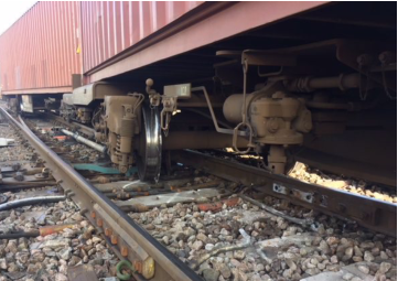 (1) Flange climbing
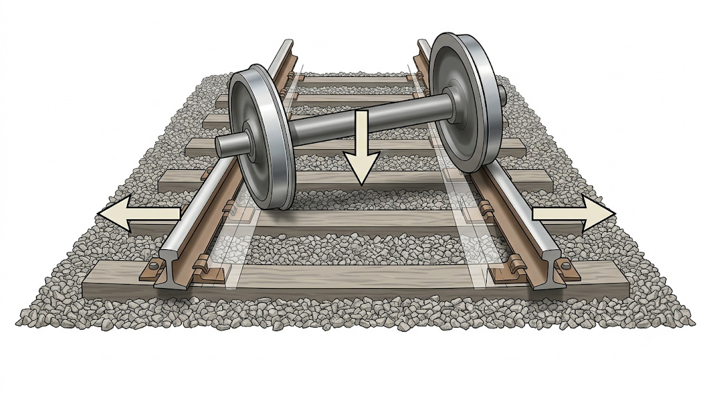 (2) Gauge spreading
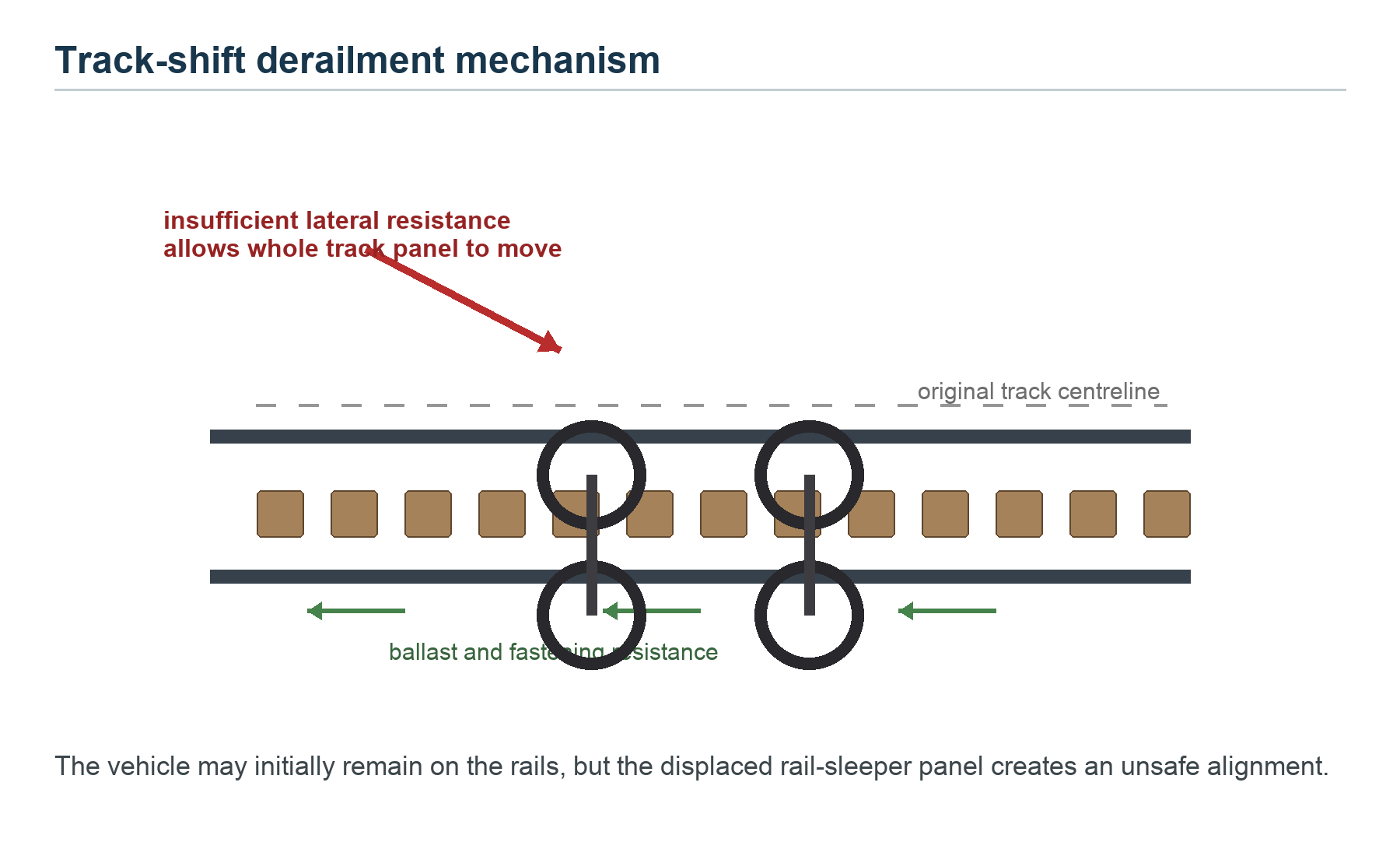 (3) Track shifting
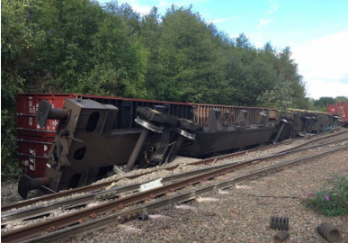 (4) Vehicle overturn
On 15 February 2012, northbound train 12926 derailed near Nykirke station on the Vestfold line (Figure 8.12). The accident investigation found that the train was travelling too fast for the section after a speed reduction from 130 to 70 km/h before a curve [1]. The case illustrates that derailment risk is not only a wheel–rail contact issue; operating speed, speed-control barriers and route knowledge can also be decisive.
![Train derailment near Nykirke station on the Vestfold line, 15 February 2012 [1].](../../assets/chapters/ch08/original/figures_lecture_crops/fig_derailment_photo_context_4x3.jpg)
8.6.2 Flange-Climbing Mechanism
During incipient flange climbing, the contact normal and friction force are resolved into vertical and lateral components. The force sketch in Figure 8.13 defines the quantities used in the Nadal derivation: vertical wheel load \(Q\), lateral force \(Y\), contact normal \(N\), flange angle \(\beta\) and friction coefficient \(\mu\).
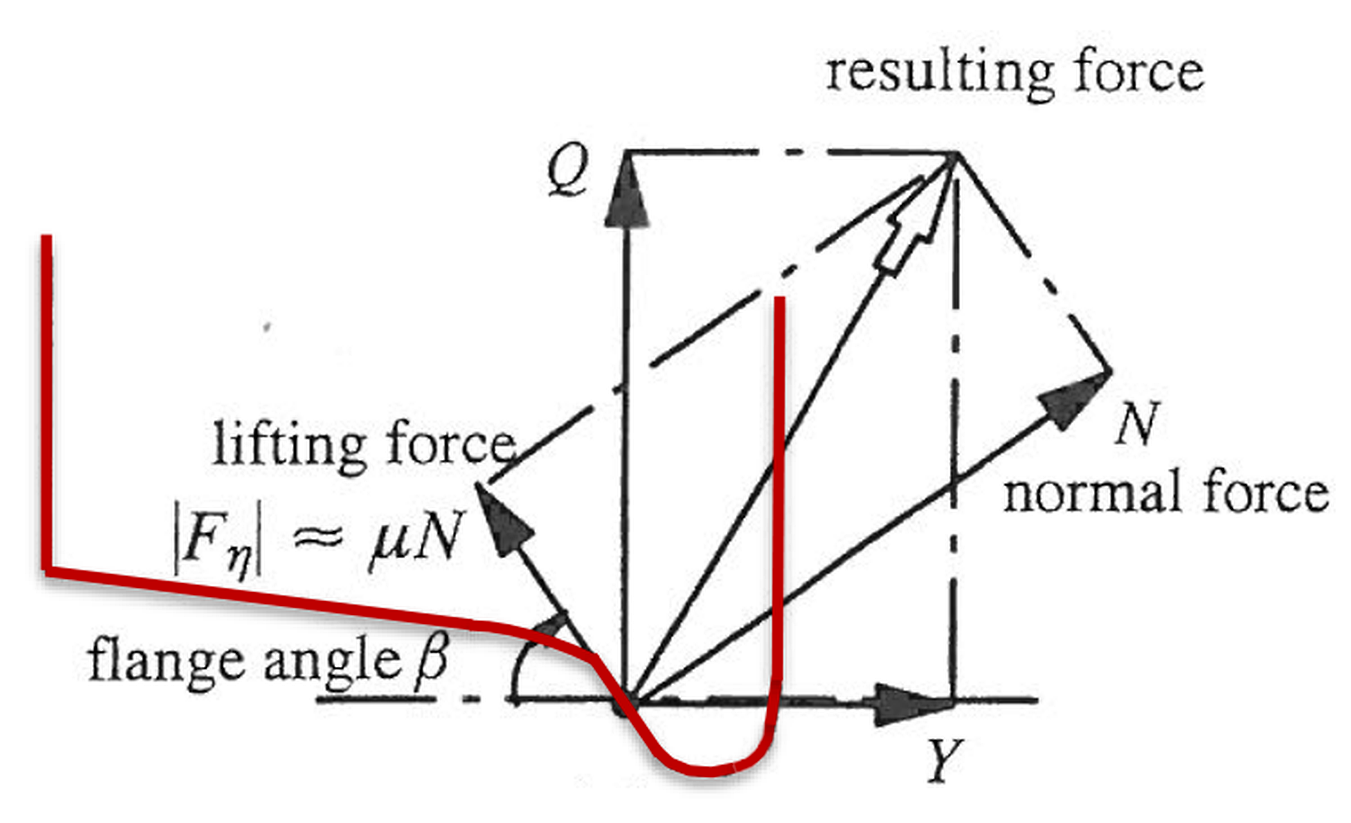
Flange climbing proceeds in three phases:
-
Under a lateral force, the wheel moves toward the rail and makes flange contact. A creep force at the contact point initially opposes climbing.
-
As the flange angle increases, the lateral component of the creep force reverses and begins to assist climbing.
-
Once the wheel passes the maximum contact angle, the creep force reverses again, but by then the wheel may already be climbing over the rail head.
Three basic conditions promote flange climbing:
-
A large lateral force \(Y\) pushing the wheel toward the rail.
-
A high \(Y/Q\) ratio, i.e. large lateral force combined with a reduced vertical load \(Q\) on the flanging wheel.
-
A positive angle of attack of the wheelset on the rail (yaw angle), which generates additional lateral force.
In the stage sketch, the three panels correspond to the numbered phases above: initial flange contact, creep-force reversal and the final climb-over risk (Figure 8.14).

8.6.3 Nadal Criterion
The Nadal criterion [113, 65] gives the limiting lateral-to-vertical force ratio \((Y/Q)\) at which flange climbing begins. The word limit means an upper allowable value: if the actual wheel force ratio is below the limit, flange climbing is not predicted by the simple criterion; if it reaches or exceeds the limit, incipient climb is indicated. Resolving forces at the wheel–rail contact point on the flange:
Dividing:
where \(\beta\) is the flange angle (measured from the vertical) and \(\mu\) is the coefficient of friction. Flange climbing is imminent when:
The number is not universal because it depends on contact angle and friction. For example, with \(\mu=0.35\):
Thus a measured \(Y/Q=0.6\) is below these limits, whereas \(Y/Q=0.9\) would exceed a limit of about 0.8 and would be critical for that assumed contact condition. Key observations:
-
A lower flange angle \(\beta\) reduces the limiting \(Y/Q\), making climbing easier. Modern flange angles are typically \(60\)–\(70^\circ\).
-
A higher friction coefficient \(\mu\) reduces the limiting \(Y/Q\) because friction assists the climbing once the creep force reverses.
-
Nadal's criterion is conservative for small or negative angles of attack.
8.6.4 Weinstock Criterion
The Weinstock criterion [166, 153] is an axle-level wheel-climb safety check. It extends the Nadal idea by using information from both wheels of the same axle. Define the Nadal single-wheel limit as
For an axle, the Weinstock check uses the axle-sum derailment ratio
where subscript \(f\) denotes the flanging wheel and \(n\) the non-flanging wheel. The limiting axle-sum value is commonly written as
and flange-climbing risk is indicated when \(S_{Y/Q}\) exceeds this limit. The additional \(\mu\) term represents the contribution that can be inferred from the non-flanging wheel. For this reason, Weinstock is usually less conservative than a single-wheel Nadal check when the axle motion and the forces on both wheels are considered.
The Nadal and Weinstock values are theoretical wheel-climb limits because they come from simplified contact-force equilibrium. In vehicle running-dynamics acceptance, EN 14363 and UIC Code 518 [87, 159] also use conservative measured-force limits. These limits should be understood as requirements on a processed measurement signal, not simply on one raw instantaneous sample. For a single wheel, define
where the overbar denotes a moving average over a 2 m distance window and the maximum is taken over the relevant test zone. A commonly quoted large-radius running-safety check is
In UIC 518 this is commonly associated with large-radius conditions such as \(R\geq300\) m. Exact radius classes, filtering, statistical treatment and pass/fail wording depend on the applied standard and national rules, so the processing definition should be stated together with the numerical limit. A value below 0.8 passes this particular measured-force screening check, while a value above 0.8 exceeds it. Because the averaging window is distance-based, its time duration is \(t_{2m}=2/v\): at 40 km/h it is about 0.18 s, while at 160 km/h it is about 0.045 s. Some rules express short impulses by duration instead, for example by treating exceedances shorter than about 50 ms differently from sustained values. A raw spike, a 2 m moving-mean maximum and a duration exceedance are therefore not equivalent signals. The practical 0.8 limit is not a new flange-contact formula; it is a conservative operational screening limit used alongside the Nadal and Weinstock calculations and other running-safety checks.
Worked example (Nadal and Weinstock checks).
Assume a flange angle \(\beta=70^\circ\) and friction coefficient \(\mu=0.35\). The single-wheel Nadal limit is
and the corresponding Weinstock axle-sum limit is
Consider an axle where the non-flanging wheel carries \(Y_n=25\) kN and \(Q_n=90\) kN. The table compares two states of the flanging wheel:
| Case | \(Y_f\) [kN] | \(Q_f\) [kN] | \(Y_f/Q_f\) | \(S_{Y/Q}\) |
|---|---|---|---|---|
| Nominal wheel load | 70 | 75 | 0.93 | \(0.93+25/90=1.21\) |
| Unloaded wheel | 70 | 50 | 1.40 | \(1.40+25/90=1.68\) |
The nominal case is below both theoretical limits. With the same lateral force but a reduced vertical wheel load, the flanging wheel exceeds the Nadal limit and the axle-sum ratio also exceeds the Weinstock limit. This simple comparison is why wheel unloading from twist, cant excess or vehicle roll is so important in derailment assessment.
8.6.5 Risk Factors for Flange Climbing
Flange climbing risk is governed more by low vertical wheel load \(Q\) than by high lateral force \(Y\). The key risk factors are:
Vehicle-related.
-
Light, torsionally stiff vehicles (e.g. empty tank wagons) are most vulnerable because torsional rigidity concentrates unloading on one wheel when the track is twisted.
-
High angles of attack increase lateral force and thus \(Y/Q\).
-
Vehicle hunting generates large cyclic lateral forces.
Track-related.
-
Cant excess: if the vehicle speed is lower than the balanced speed, the outer wheel load is reduced.
-
Track twist beyond tolerances severely unloads one wheel.
-
Switches and crossings impose sudden profile changes.
Environmental.
-
Inward wind reduces vertical wheel load and simultaneously increases the lateral force on the windward side.
-
Contamination (ice, sand, oil) alters the friction coefficient.
Preventive measures.
-
Limit track cant in tight curves to prevent cant excess at low vehicle speeds.
-
Enforce track twist tolerances (typically \(\leq 3\) mm per metre for high-speed lines).
-
Apply flange or rail lubrication at critical locations.
-
Coordinate vehicle suspension stiffness with track curvature.
8.7 Chapter Summary
Contact patch. The small contact area between wheel and rail must support the vehicle, guide the wheelset, transmit traction and braking forces and resist lateral derailment. The contact stress is high because the load is concentrated, and the contact position changes with wheel profile, rail profile, curvature, cant and vehicle motion. This makes wheel–rail interaction one of the most important coupled problems in railway engineering.
Conicity. A conical wheelset can steer itself because a lateral displacement creates a rolling-radius difference between the two wheels. Klingel's formula describes the resulting sinusoidal motion and shows how wavelength depends on wheel radius, gauge and equivalent conicity. Although the model is idealised, it explains why profile shape matters for both curving behaviour and straight-track stability.
Hunting stability. At higher speeds, the self-steering mechanism can become unstable and develop hunting motion. The critical speed depends on wheel and rail profiles, suspension stiffness and damping, vehicle mass distribution and contact conditions. A wheel profile that gives good guidance in curves can also increase equivalent conicity and reduce hunting stability on tangent track, so profile design requires compromise.
Contact mechanics. Hertzian contact theory estimates the size and pressure distribution of the contact patch, while tangential contact governs creep forces, traction, braking and curving. The limitations of these models are important: real rail and wheel surfaces are worn, rough, contaminated and sometimes plastically deformed. Still, the models provide the engineering language needed to discuss rail fatigue, wear and adhesion.
Derailment safety. Flange climbing occurs when lateral force and vertical unloading allow the wheel flange to climb the rail. Nadal's criterion and the Weinstock approach relate this risk to the ratio of lateral and vertical wheel forces, contact angle and friction. These criteria do not replace full vehicle dynamics, but they give practical checks for curves, switches, degraded track and other locations where derailment resistance is critical.
Assignments
Assignment 1: Wheelset guidance in curves and straight track
A wheelset has nominal rolling radius \(r_0=460\) mm, contact half-spacing \(b_0=750\) mm and equivalent conicity \(\lambda_{eq}=1/20\).
(a) Starting from the rolling-radius relation \(r_\mathrm{out}=r_0+\lambda_{eq}y\) and \(r_\mathrm{in}=r_0-\lambda_{eq}y\), derive the lateral displacement needed for radial steering:
(b) Calculate \(y_R\) for curve radii \(R=500\) m and \(R=250\) m. If only about 8 mm of tread displacement is available before flange contact, discuss whether pure rolling is possible in the two curves.
(c) Starting from the total rolling-radius difference \(\Delta r = 2\lambda_{eq}y\) and \(\mathrm{d}\psi/\mathrm{d}x=-\Delta r/(2b_0r_0)\), derive the Klingel differential equation for straight-track motion.
(d) Calculate the Klingel wavelength and the kinematic hunting frequency at \(v=200\) km/h. Then explain the practical trade-off between low and high equivalent conicity.
Assignment 2: Hunting stability and limit-cycle curves
The hunting-stability diagram relates vehicle speed to the lateral oscillation amplitude of the wheelset or vehicle. It includes stable regions, a conditionally stable region, an unstable region, a nonlinear critical speed \(v_\mathrm{crit,nonlin}\), a linear critical speed \(v_\mathrm{crit,lin}\), and a limit-cycle branch.
(a) Explain what the two axes of the limit-cycle curve represent, and what the limit-cycle branch means physically.
(b) Explain why a large lateral disturbance can trigger hunting below the linear critical speed, and why this matters for wheel–rail interaction assessment.
(c) Propose at least two ways to avoid unstable hunting oscillation.
(d) Explain why a very stiff primary suspension can be unfavourable for curve negotiation even if it improves straight-track guidance.
Assignment 3: Wheel–rail contact problem
Use the Hertzian contact equations in this chapter. Assume tangent track (\(r_{x2}\rightarrow\infty\)), a static axle mass of \(22.5\,\mathrm{t}\) and Poisson's ratio \(\nu=0.283\) unless otherwise stated. Use Table 8.1 to obtain the Hertz constants \(m\) and \(n\). The corresponding static axle load is \(220.7\,\mathrm{kN}\), so the normal force per wheel may be taken as \(N=110.4\,\mathrm{kN}\).
Contact cases for the Hertz calculation
| Case | Wheel diameter | \(r_{y1}\) | \(r_{y2}\) | Elastic modulus |
|---|---|---|---|---|
| 1 | 920 mm | 150 mm | 300 mm | \(E_w=E_r=210\) GPa |
| 2 | 920 mm | 150 mm | 300 mm | \(E_w=180\) GPa, \(E_r=210\) GPa |
| 3 | 920 mm | \(-200\) mm | 80 mm | \(E_w=E_r=210\) GPa |
| 4 | 750 mm | \(-200\) mm | 80 mm | \(E_w=E_r=210\) GPa |
(a) List the assumptions behind Hertzian contact theory.
(b) For each case, calculate \(A\), \(B\), the combined elastic modulus \(E^*\), the contact semi-axes \(a\) and \(b\), the contact area \(A_c\), and the maximum contact pressure \(P_{z,\max}\).
(c) Compare Case 2 with Case 1, Case 3 with Case 1, and Case 4 with the gauge-corner Case 3. What do these comparisons say about material stiffness, contact location and wheel diameter?
(d) At a low-friction condition \(\mu=0.2\), explain how the tangential creep-force vector is limited by the friction bound \(\sqrt{X^2+Y^2}\leq \mu N\). What happens when the linear creep-force demand exceeds this bound?
Assignment 4: Nadal and Weinstock derailment criteria
Focus only on flange-climbing derailment at the wheel–rail interface.
(a) Plot, or prepare a table for, the Nadal and Weinstock \(Y/Q\) limits as a function of flange contact angle \(\beta\) from \(20^\circ\) to \(80^\circ\). Use friction coefficients \(\mu=0.1,0.2,0.3,0.4,0.5\).
(b) Comment on the difference between the Nadal and Weinstock criteria. Why is Nadal usually more conservative?
(c) Discuss how flange/rail lubrication affects flange-climbing derailment risk.
(d) For \(\beta=70^\circ\), \(\mu=0.35\), measured lateral force \(Y=55\) kN and vertical force \(Q=100\) kN, calculate the measured \(Y/Q\) ratio and compare it with the Nadal limit and a common EN 14363/UIC 518 measured-force screening check based on a 2 m moving mean, \(D_{Y/Q}\leq0.8\).