01

Trafikkbelastning på jernbanespor

Kort videoforklaring Se video

1.1 Innledning

En jernbane er et styrt transportsystem der kjøretøy beveger seg langs et par faste stålskinner. I motsetning til veitransport er grensesnittet mellom stålhjulet og stålskinnen geometrisk og mekanisk styrt: Skinnehodets profil styrer hjulet sideveis, mens skinnen må bære og fordele vertikalkrefter, langsgående krefter og tverrkrefter fra passerende tog [68]. Kontaktflaten er vanligvis mindre enn en tommelfingernegl, men overfører likevel lasten fra ett hjul om gangen. Ved en aksellast på 30 t overfører hver hjulkontakt omtrent 147 kN. Trafikklastene på jernbanespor er dermed blant de mest konsentrerte og hyppigst gjentatte lastene innen bygg- og anleggsteknikk.

Trafikklaster på jernbanespor omfatter alle krefter og lastvirkninger som jernbanekjøretøy påfører sporinfrastrukturen når de står stille eller er i bevegelse. I dette kapitlet brukes trafikklast om den fysiske lasten fra tog, mens trafikkbelastning brukes om akkumulert trafikkmengde eller årlig bruttotonnasje. En grundig forståelse av disse størrelsene er nødvendig i alle deler av jernbaneteknikken:

• Dimensjonering av spor: Lastberegningene styrer valget av skinneprofil, svilletype og svilleavstand, befestigelsessystem og nødvendig ballastdybde.

• Dimensjonering av bruer og konstruksjoner: Standardiserte lastmodeller (f.eks. lastmodell LM71 i EN 1991-2) er utviklet på grunnlag av statistikk for trafikklaster.

• Vedlikeholdsplanlegging: Hastigheten på nedbrytningen av sporgeometrien er direkte knyttet til trafikkbelastningen; tyngre og raskere tog bryter ned sporet raskere.

• Sikkerhetsvurdering: For høye spenninger i skinne eller ballast kan føre til skinnebrudd, solslyng eller svikt i undergrunnen, som alle kan være mulige årsaker til avsporing.

Trafikklaster på jernbanespor deles etter fysisk opprinnelse inn i tre grupper [130]:

1. Statiske laster: Tyngdekrefter fra egenvekten til et stillestående kjøretøy, som bestemmes fullt ut av aksellastfordelingen.

2. Kvasistatiske laster: Langsomt varierende krefter som oppstår når et tog kjører gjennom en horisontalkurve (sentrifugalkraft) eller utsettes for sidevind. Kreftene fører til omlagring av last mellom inner- og ytterskinne og mellom boggiene.

3. Dynamiske laster: Hurtig varierende krefter som skyldes ujevnheter i sporet (rifler, skinneskjøter og sporveksler), feil på kjøretøyet (hjulslagflater og urunde hjul) og hastighetsavhengige resonanser i kjøretøy–spor-systemet. Dynamiske laster kjennetegnes av statistisk variasjon og ivaretas vanligvis ved hjelp av en dynamisk forsterkningsfaktor (DAF).

Dette kapitlet innfører UIC-systemet for klassifisering av akselrekkefølge, mekanismene for lastfordeling gjennom sporkonstruksjonen og Eisenmanns analytiske metode for beregning av statiske og dynamiske spenninger i skinner, sviller og ballast. Kapitlet viser gjennomgående til kravene i Bane NORs tekniske regelverk [10] og Bane NORs Network Statement [30].

1.2 Jernbanesystemer og belastningsforhold

Begrepet «jernbane» omfatter et bredt spekter av styrte transportsystemer med svært forskjellige kjøretøymasser, aksellaster og driftshastigheter. Belastningsforholdene bestemmes av banens driftsformål, og de må forstås før en konstruksjonsanalyse kan gjennomføres. Det skilles mellom tre hovedkategorier [130]:

1.2.1 By- og nærtrafikkbaner

By- og nærtrafikkbaner omfatter T-bane, bybane og trikk. Systemene dekker en stor etterspørsel etter persontransport i byområder og kjøres med korte intervaller over forholdsvis korte avstander. De viktigste egenskapene er:

• Aksellaster vanligvis i området 8–15 t

• Maksimalhastigheter vanligvis 80–120 km/h

• Egen infrastruktur (i de fleste tilfeller atskilt fra veitrafikk)

• Høy avgangsfrekvens, som krever et robust spor med lite vedlikeholdsbehov

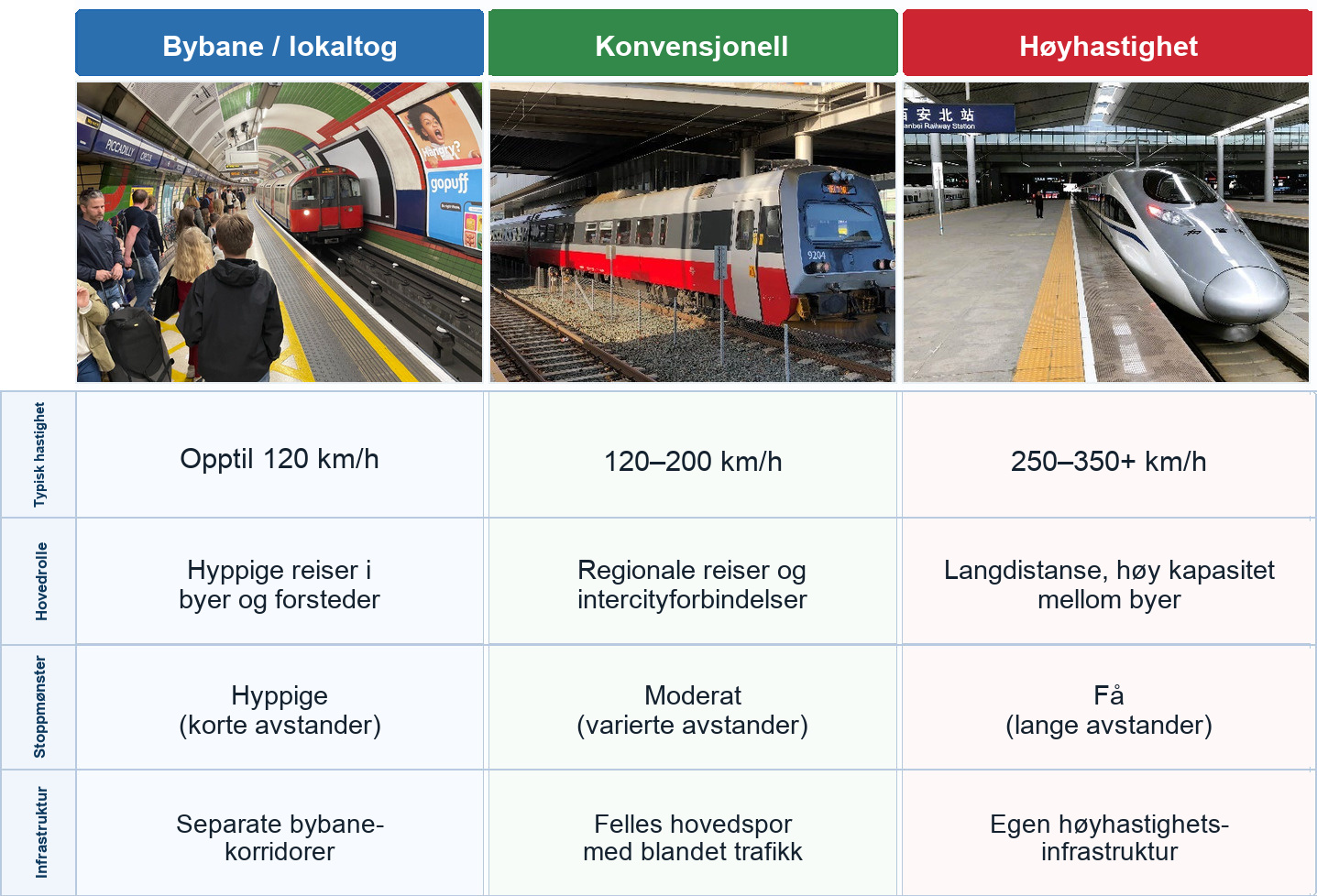
Sammenligningen i Figur 1.1 skal leses kvalitativt og ikke som et bindende dimensjoneringsdiagram. By- og nærtrafikkbaner kjennetegnes av hyppige stopp og forholdsvis lave til moderate aksellaster. Konvensjonelle systemer og høyhastighetssystemer vises som kontraster med høyere driftshastigheter, større avstand mellom stasjonene og strengere krav til atskilt infrastruktur. Det sentrale jernbanetekniske poenget er at den dimensjonerende problemstillingen endres med driftskonseptet: Bysystemer begrenses av stasjonsavstand, tunneler, konstruksjoner og gatespor eller kompakte sporløsninger, mens konvensjonelle baner og høyhastighetsbaner må oppfylle konstruksjonsmessige, dynamiske og geometriske krav til hovedbaner.

Figur 1.1 Kategorier av jernbanesystemer for persontrafikk og typiske driftsegenskaper.

1.2.2 Konvensjonelle jernbaner

Konvensjonelle jernbaner fører både fjerntog for persontrafikk og godstog, vanligvis på felles infrastruktur. De utgjør ryggraden i det nasjonale jernbanenettet. Belastningsforholdene varierer mye:

• Aksellaster for persontog: vanligvis 12–22,5 t; aksellaster for godsvogner: normalt 20–22,5 t på europeiske hovedbaner med standard belastning

• Maksimalhastigheter: opptil 210 km/h for persontog i Norge; vanligvis 80–120 km/h for godstog, med strekningsspesifikke begrensninger (Bane NOR Network Statement 2026 [30]; ytelseskategorier i TSI Infrastruktur [71])

• Blandet trafikk krever spor som er dimensjonert både for høy hastighet og høy aksellast

Det resulterende avveiningsforholdet mellom aksellast og driftshastighet er skjematisk oppsummert i Figur 1.2.

Figur 1.2 Skjematiske områder for aksellast og hastighet ved konvensjonell jernbanedrift. Standard europeisk godstrafikk er vist med omtrent 20–22,5 t per aksel, mens høyhastighetstog for persontrafikk har forholdsvis lave aksellaster ved vesentlig høyere hastigheter [71, 70, 169].

1.2.3 Spesialiserte jernbanesystemer

Enkelte jernbanesystemer er utviklet for ett bestemt formål, og belastningsforholdene skiller seg vesentlig fra konvensjonelle jernbaner:

• Høyhastighetsbaner: Egne baner for persontrafikk (f.eks. TGV i Frankrike og Shinkansen i Japan) med hastigheter over 250 km/h. Aksellastene er forholdsvis lave (12–17 t), men dynamiske virkninger ved høy hastighet er dimensjonerende.

• Baner for tung godstrafikk: Godsbaner med aksellaster vesentlig over standardverdien på 22,5 t, vanligvis for transport av bulkvarer (jernmalm, kull og korn). Ofotbanen i Nord-Norge fører jernmalmtrafikk med strekningsspesifikke godkjenninger for høye aksellaster; malmtrafikken benytter vanligvis aksellaster på 30 t, mens Bane NOR også angir egne klassegrenser for bestemte kjøretøykategorier og hastigheter på Ofotbanen [30].

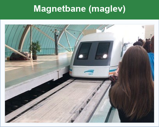
• Magnetisk levitasjon (maglev): Høyhastighetssystemer som drives og styres av elektromagnetiske krefter uten fysisk hjul–skinne-kontakt. Maglev skaper ikke kontaktspenninger mellom hjul og skinne, men føringsbanen må likevel motstå betydelige aerodynamiske og magnetiske krefter.

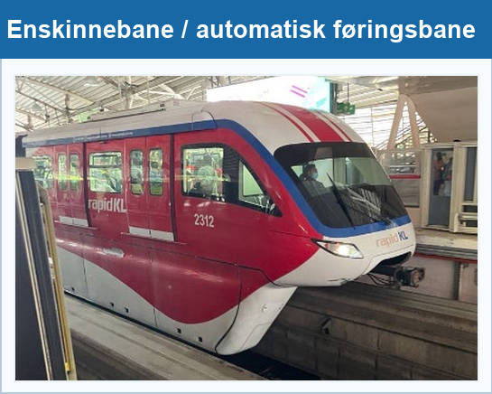
• Andre styrte systemer: Énskinnebaner, automatiske persontransportsystemer, kabelbaner og tannstangbaner utformes ofte rundt et eget konsept for føringsbane, trekkraft eller bremsing i stedet for det vanlige grensesnittet mellom stålhjul og to skinner.

Tre eksempler tydeliggjør hvorfor spesialiserte jernbanesystemer må behandles separat fra vanlige spor med to skinner:

• Énskinnebaner og automatiske føringsbanesystemer går på en egen bjelke eller føringsbane. Den konstruktive lastoverføringen bestemmes derfor av føringsbjelken og bæresøylene i stedet for av samvirket mellom skinne, sville og ballast.

• Maglevsystemer bruker elektromagnetisk opplagring, styring og fremdrift. De skaper ikke kontaktspenninger mellom hjul og skinne, men føringsbanen må bære magnetiske og aerodynamiske krefter samt bremse- og kjøretøylaster.

• Kabelbaner og fjellbaner er utformet for bratte stigninger. Kabeltrekk, bremsesystemer og lokal geometri i føringsbanen blir sentrale dimensjoneringsforhold.

Felles for disse spesialiserte systemene er at lastoverføringsmekanismen er systemspesifikk og ikke styres av det konvensjonelle hjul–skinne-grensesnittet.

Figur 1.3 Eksempler på spesialiserte jernbanesystemer.(a) énskinnebane og automatbane; (b) magnetbane (maglev); og (c) kabelbane og fjellbane.

1.3 Klassifisering av akselrekkefølge

Antallet aksler og plasseringen av dem på et lokomotiv eller motorvognsett bestemmer hvordan kjøretøyets samlede masse fordeles på sporet. Hjulrekkefølgen eller akselrekkefølgen er derfor en grunnleggende parameter i enhver analyse av trafikkbelastning.

Tre hovedsystemer for klassifisering brukes internasjonalt [115, 148]:

1. AAR-systemet, som brukes i Nord-Amerika for diesel- og elektriske lokomotiver.

2. Whyte-notasjonen, som historisk ble brukt i Nord-Amerika og Storbritannia for damplokomotiver.

3. UIC-klassifiseringen (også kalt det tyske systemet), som brukes i det kontinentale Europa, inkludert Norge.

1.3.1 UIC-systemet for akselrekkefølge

UIC-klassifiseringen forvaltes av Den internasjonale jernbaneunionen (UIC) og er standardisert i IRS 60650 [115]. Klassifisering av baner for vedlikeholdsformål følger UIC 714 [169]. Notasjonen er bygd opp av følgende elementer:

• Store bokstaver angir grupper av drivaksler: A = 1 drivaksel, B = 2 drivaksler, C = 3 drivaksler, D = 4 drivaksler og så videre.

• Liten «o» etter en stor bokstav angir at hver aksel i gruppen har sin egen trekkmotor (f.eks. betyr «Bo» to drivaksler med hver sin motor). Uten «o» er akslene i gruppen mekanisk koblet sammen.

• Arabiske tall angir grupper av løpeaksler uten drift: 1 = 1 løpeaksel, 2 = 2 løpeaksler osv.

• Apostrof (\('\)) etter en bokstav eller et tall angir at den aktuelle akselgruppen er montert i en dreibar boggi i stedet for direkte i hovedrammen.

• Parenteser grupperer bokstaver og tall som beskriver samme boggi, og gjør apostrofen overflødig som angivelse av boggimontering.

• Plusstegn (+) skiller permanent sammenkoblede, men mekanisk uavhengige trekkenheter i samme lokomotiv eller togsett.

1.3.2 Vanlige UIC-akselrekkefølger

Grunngrupper (uten boggi):

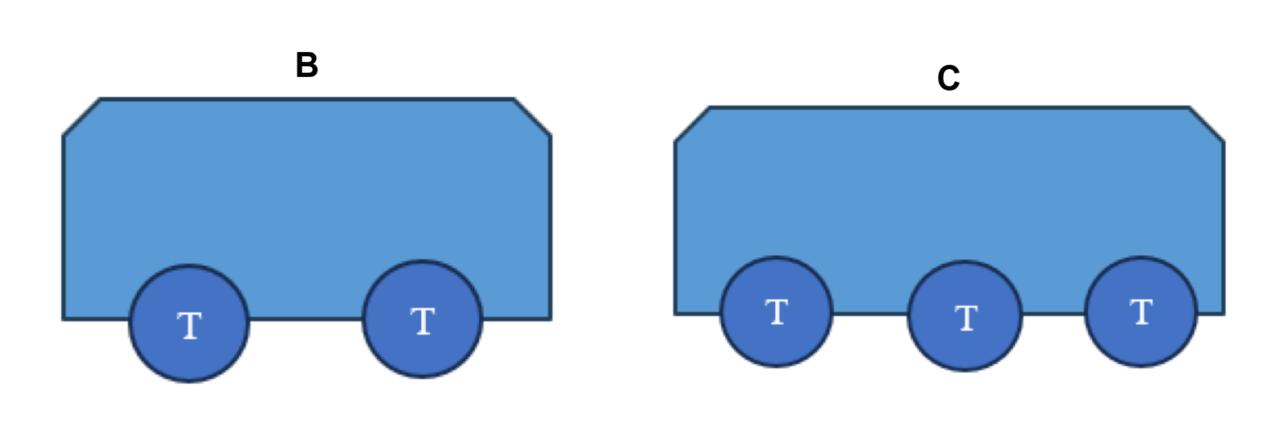
I de enkleste akselrekkefølgene er akslene montert direkte i hovedrammen, som vist i Figur 1.4 for «B» (to sammenkoblede drivaksler) og «C» (tre sammenkoblede drivaksler). Disse løsningene med stiv ramme overfører aksellastene direkte i faste posisjoner langs rammen. I skissene som brukes her, markerer \(T\) en drivaksel.

Figur 1.4 Grunngrupper av drivaksler i UIC-systemet: B har to drivaksler, og C har tre drivaksler.

Akselrekkefølger med boggier:

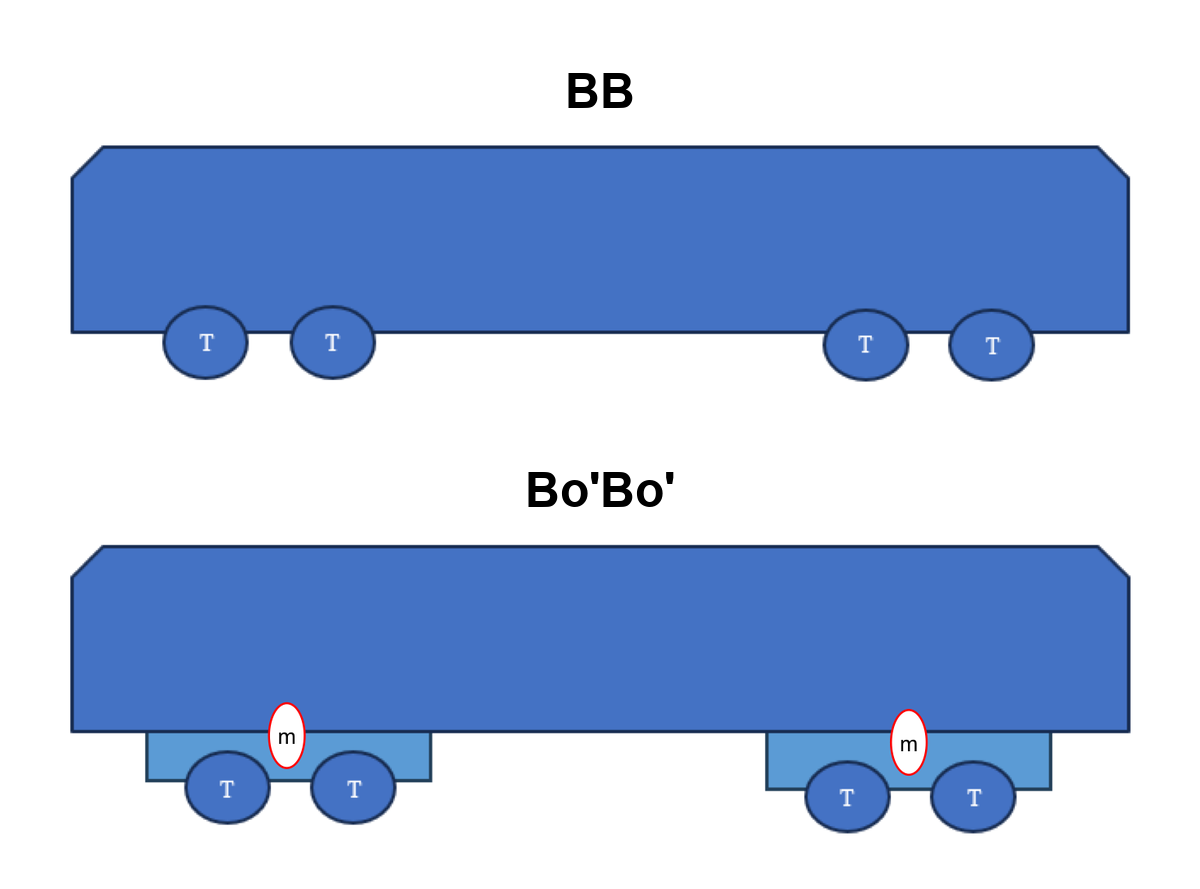
Moderne lokomotiver bruker nesten alltid boggier. En boggi er en underramme som bærer to eller flere aksler og dreier under vognkassen, slik at lokomotivet kan kjøre gjennom kurver uten å påføre skinnene store sidekrefter. Forskjellen er konstruktivt viktig: I Figur 1.5 har BB fire drivaksler fast montert i hovedrammen, mens Bo'Bo' plasserer de fire drivakslene i to boggier med individuelle motorer. Den røde \(m\) i figuren markerer trekkmotorene.

Figur 1.5 Sammenligning av BB og Bo’Bo’. Apostrofen angir boggimontering; «o» angir individuelt drevne aksler.

Lengre akselrekkefølger:

Seksakslede lokomotiver er vanlige ved stor ytelse eller tung godstrafikk. Derfor er Co'Co'-rekkefølgen i Figur 1.6 mye brukt i godstrafikk med stor ytelse og i blandet trafikk. Figuren viser også to lengre eksempler: Bo'A1A, der én gruppe inneholder en løpeaksel, og Bo'2'2' + 2'Bo', der plusstegnet skiller to permanent sammenkoblede, men mekanisk uavhengige enheter.

Figur 1.6 Flere UIC-eksempler: Co’Co’, Bo’A1A og Bo’2’2’ + 2’Bo’. Hjulsatser uten betegnelse representerer løpeaksler.

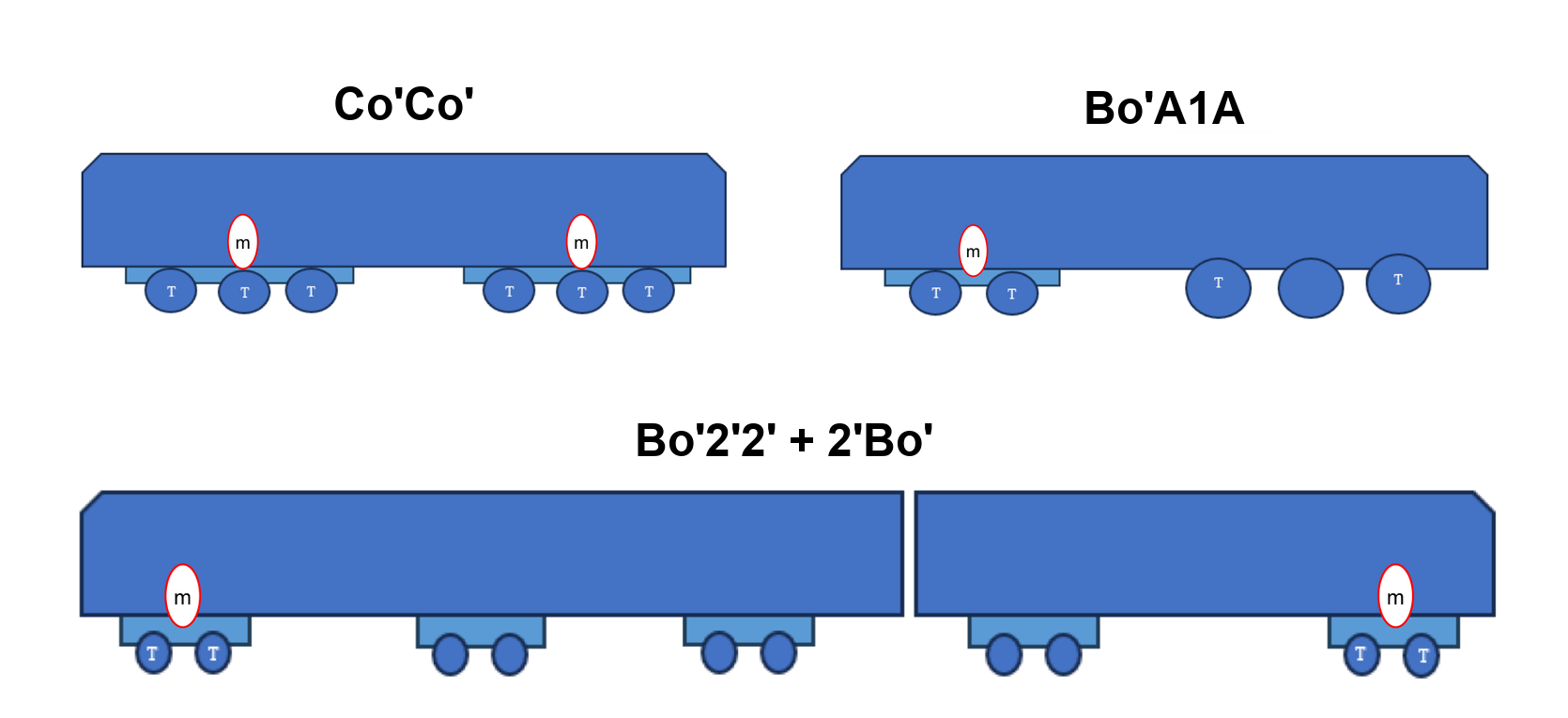
Eksemplene ovenfor kan leses som kompakte notasjonsregler: Bokstavene beskriver akselgrupper, apostrofene viser boggimontering, og «o» markerer aksler med hver sin motor.

Notasjon	Beskrivelse
B	2 drivaksler, montert i rammen og mekanisk koblet sammen
Bo'	2 drivaksler, montert i boggi og drevet av hver sin motor
BB	4 drivaksler montert i rammen
Bo'Bo'	4 drivaksler i 2 boggier med to aksler, drevet av hver sin motor
Co'Co'	6 drivaksler i 2 boggier med tre aksler, drevet av hver sin motor
Bo'A1A	4 drivaksler og 1 løpeaksel; én boggi med to drivaksler og én gruppe med tre aksler, der én er løpeaksel
Bo'Bo'Bo'	6 drivaksler i 3 boggier med to aksler (f.eks. Alstom PRIMA)
Bo'2'2' + 2'Bo'	4 drivaksler + 6 løpeaksler; to permanent sammenkoblede enheter
(1A)(A1)	4 aksler i to boggier, der de to indre er drivaksler og de to ytre er løpeaksler

Tabell 1.1 Utvalgte eksempler på akselrekkefølger i UIC-systemet.

De vanligste akselrekkefølgene på moderne europeiske lokomotiver er i dag Bo'Bo' (fireakslede elektriske og dieselelektriske lokomotiver for blandet trafikk eller persontrafikk) og Co'Co' (seksakslede lokomotiver med stor ytelse eller for tung godstrafikk). Betegnelsen bestemmer trekkraftytelsen og hvordan lastene fordeles på sporet. Dette påvirker direkte spenningene som beregnes i Avsnitt 1.5.

1.4 Lastfordeling gjennom sporkonstruksjonen

I dette avsnittet følges den vertikale hjullasten fra kontaktpunktet på skinnen og ned gjennom svillene, ballasten og det bærende formasjonsplanet. Det sentrale dimensjoneringsspørsmålet er hvordan hvert lag fordeler lasten før den når neste lag.

1.4.1 Aksellast og hjullast

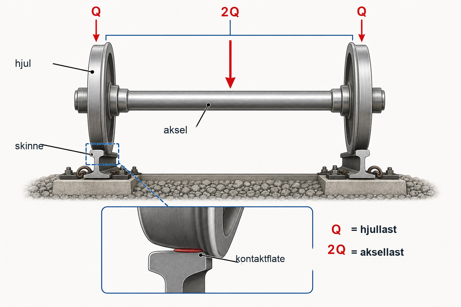
I jernbaneteknikk standardiseres kjøretøybelastningen ved hjelp av aksellasten \(P\), som er den samlede vertikale kraften én komplett aksel (begge hjulene til sammen) påfører skinnene. Hjullasten \(Q\) er andelen som bæres av ett hjul. Ved symmetrisk belastning (som gjelder på rett spor) er:

\[ Q = \frac{P}{2} \]

(1.1)

I kurver fører sentrifugalkraft og manglende overhøyde til at ytterhjulet bærer en større last enn innerhjulet. Denne kvasistatiske omlagringen av hjullast behandles i Avsnitt 1.6; skissen av hjulsatsen nedenfor innfører notasjonen med to hjul og to skinner som brukes for lastfordelingen.

Figur 1.7 Skjematisk hjulsats for jernbane: To hjul er montert på en felles aksel og ruller på to skinner.

Dimensjonerende last bestemmes av kjøretøyegenskaper, linjeklassifisering og driftsbestemmelser. Typiske norske driftstilfeller spenner fra lette bybanekjøretøy til strekningsspesifikk tung malmtrafikk.

Togtype	Aksellast \(P\) [t]	Hjullast \(Q\) [kN]	Merknader
Bybane / trikk	8–12	39–59	Bysystemer
Intercity-persontog (elektrisk motorvognsett, EMU)	12–16	59–78	f.eks. Flirt, BM73
Høyhastighetstog for persontrafikk	14–17	69–83	Forholdsvis lav aksellast
Standard godsvogn	22,5	110	Europeisk standard
Tung godstrafikk (Ofotbanen)	30	147	Strekningsspesifikk malmtrafikk

Tabell 1.2 Typiske aksellaster for ulike togtyper (Bane NOR Network Statement 2026 [30]).

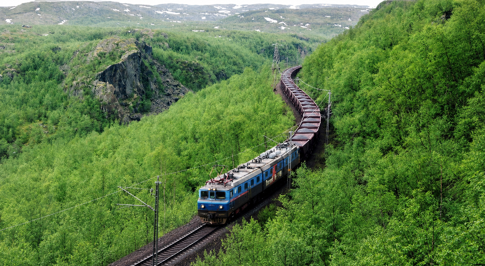
Figur 1.8 viser et malmtog på Ofotbanen/Malmbanan, som er et praktisk eksempel fra den øvre delen av aksellastområdet.

Figur 1.8 Tungt malmtog på korridoren Ofotbanen/Malmbanan, som illustrerer strekningsspesifikke høye aksellaster.

1.4.2 Komponentene i sporkonstruksjonen

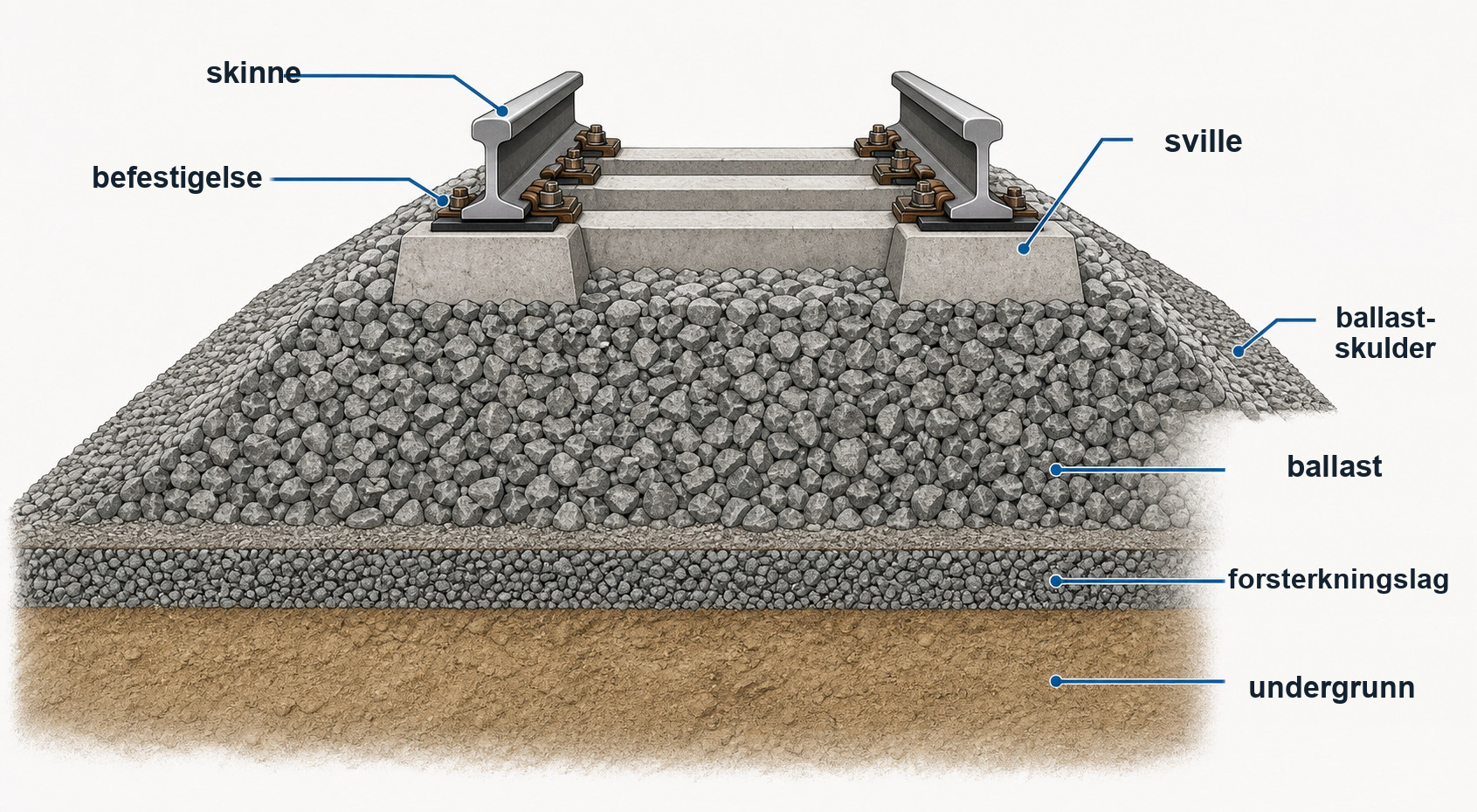
Sporkonstruksjonen består av fire hovedlag. Hvert lag fordeler og reduserer gradvis den konsentrerte hjullasten før den når undergrunnen [68, 128, 148]:

1. Skinne: Fungerer som en kontinuerlig bjelke på diskrete elastiske opplagringer (svillene). Skinnen fordeler den konsentrerte hjullasten over flere nabosviller, vanligvis tre til fem sviller totalt. Skinnens bøyestivhet \(EI_x\) bestemmer hvor langt lasten fordeles.

2. Befestigelser (skinnebefestigelser): Elastiske klemfjærer, underlagsplater og skruer som forbinder skinnen med svillen. De opprettholder skinnehelningen (vanligvis 1:20 eller 1:40), hindrer langsgående skinnebevegelse i helsveist spor og gir en viss vertikal elastisitet [88].

3. Sviller: Tverrgående elementer, vanligvis av betong, men historisk også av tre, som overfører støttepunktkreftene ved skinnesetet til ballasten, opprettholder sporvidden (\(1435\) mm i Norge) og gir sidemotstand mot solslyng.

4. Ballast: Et lag av knust, hard stein (granitt eller tilsvarende) med kontrollert kornstørrelse (vanligvis 31,5–63 mm i Norge i henhold til Bane NORs tekniske regelverk [10]); kravene til tilslag er gitt i EN 13450 [79]. Ballasten fordeler svillelastene over et stort areal av undergrunnen med en spredningsvinkel på omtrent \(45^\circ\), sørger for drenering og gjør det mulig å korrigere sporets beliggenhet ved pakking.

Den lagdelte lastoverføringen som er beskrevet ovenfor, vises skjematisk i Figur 1.9.

Figur 1.9 Skjematisk tverrsnitt av et ballastert spor med de viktigste konstruksjonslagene.

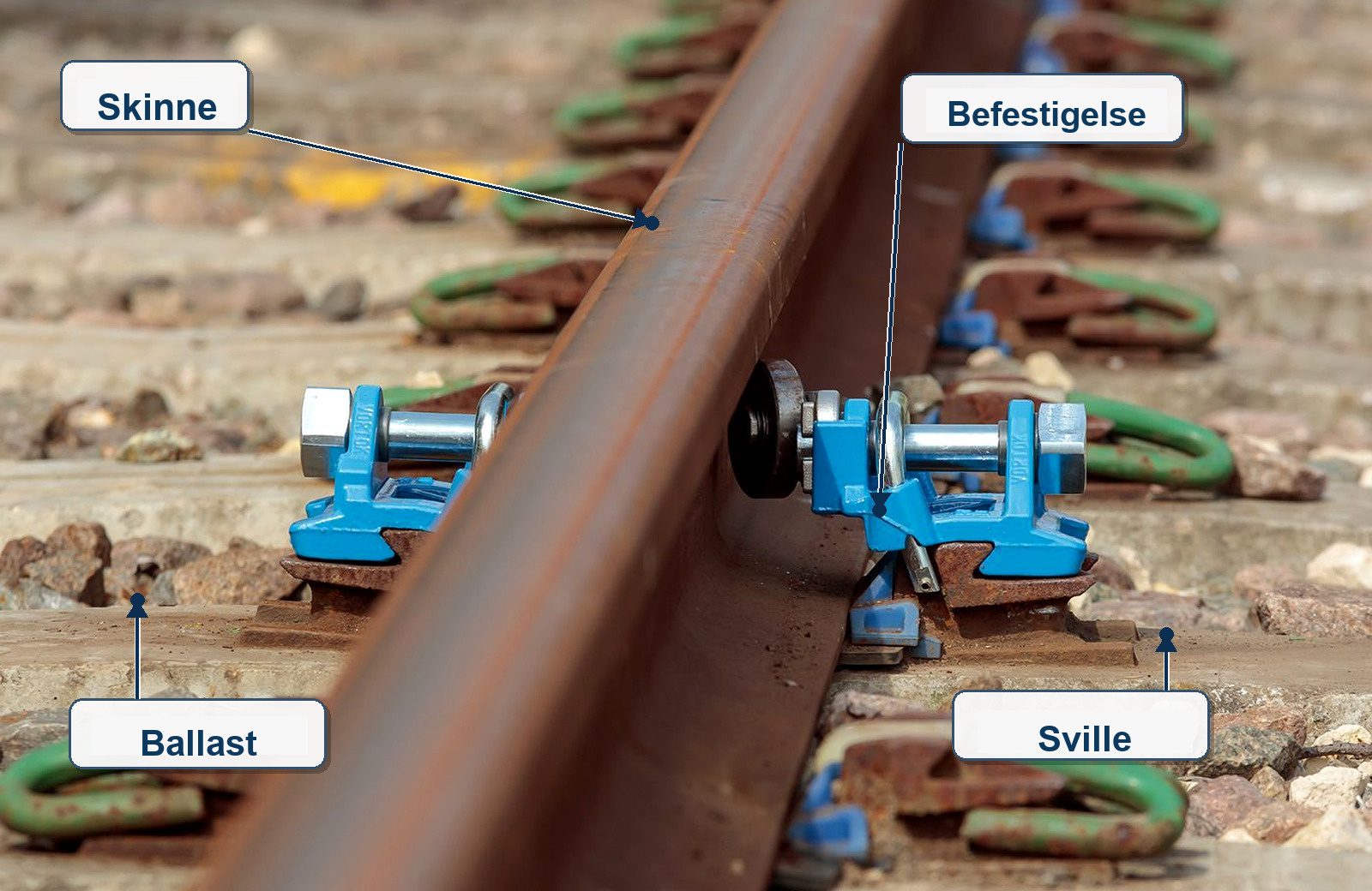
Skissen suppleres av bildet av et virkelig spor i Figur 1.10, der skinnen, befestigelsessystemet, svillen og ballasten vises i sin vanlige plassering.

Figur 1.10 Komponenter i et virkelig ballastert spor: skinne, befestigelse, sville og ballast.

1.4.3 Lastoverføring og spenningsreduksjon

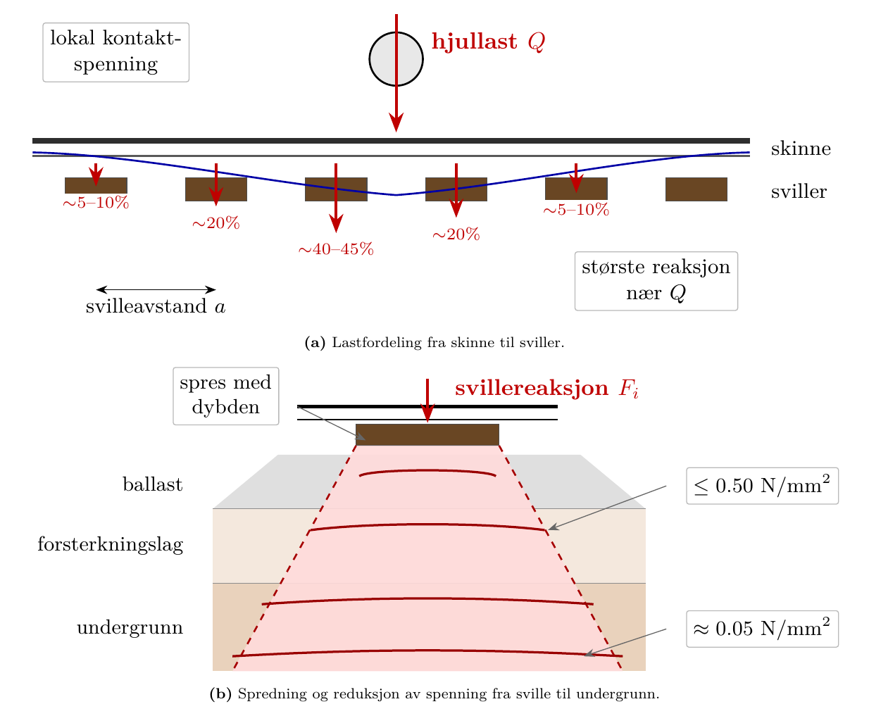
Den gradvise lastfordelingen fra hjul til undergrunn er vist i Figur 1.11. Det må skilles mellom to mekanismer. Først virker skinnen som en bjelke og fordeler én hjullast i lengderetningen til en gruppe diskrete svillereaksjoner. Den største reaksjonen oppstår vanligvis nær hjullasten. Deretter fordeler hver sville reaksjonen nedover og utover gjennom ballast, forsterkningslag og formasjonsplan. De illustrerende prosentverdiene i figuren gjelder en aksellast på 200 kN (\(Q=100\) kN) og avhenger av skinnestivhet, svilleavstand og opplagringsstivhet. Kontaktspenningen mellom hjul og skinne er svært høy: Midlere dimensjonerende kontakttrykk er vanligvis flere hundre N/mm\(^2\), og lokale maksimale kontakttrykk etter Hertz' teori kan overstige \(1000\) N/mm\(^2\) avhengig av hjullast, hjulradius og kontaktgeometri. Når lasten når overflaten av undergrunnen, er den fordelt over et areal på flere kvadratmeter, slik at spenningen reduseres til omtrent \(0{,}05\) N/mm\(^2\) (5 N/cm\(^2\)) [68].

Figur 1.11 Gradvis lastfordeling og spenningsreduksjon gjennom sporkonstruksjonen.

Den skjematiske fremstillingen i Figur 1.12 viser det samme prinsippet ved hjelp av representative kontaktarealer og spenningsnivåer i hvert grensesnitt. Figuren viser hvorfor spenningene avtar så raskt gjennom sporkonstruksjonen. Verdiene skal tolkes som størrelsesordener og ikke som dimensjoneringsgrenser.

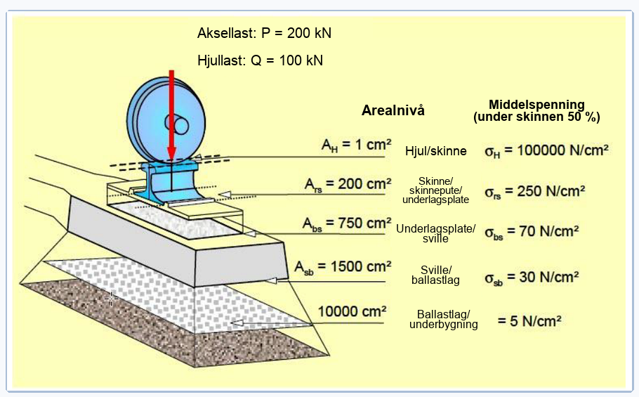
Norsk terminologi i originalfiguren: axle = aksel; wheel = hjul; area level = arealnivå; mean stress = middelspenning; wheel/rail = hjul/skinne; rail/rail pad/baseplate = skinne/skinnepute/underlagsplate; baseplate/sleeper = underlagsplate/sville; sleeper/ballast bed = sville/ballastlag; ballast bed/substructure = ballastlag/underbygning.

Figur 1.12 Representativ lastfordeling fra hjul–skinne-kontakten til formasjonsplanet.

1.4.4 Winkler-modellen for en bjelke på elastisk underlag

Skinnen modelleres analytisk som en uendelig lang bjelke på et kontinuerlig elastisk underlag, den klassiske Winkler-modellen [68]. Underlagsreaksjonen \(p\) per lengdeenhet av skinnen antas å være proporsjonal med den lokale nedbøyningen \(w\):

\[ p = k \cdot w \]

(1.2)

der \(k\) [N/mm\(^2\)] er spormodulen (underlagsstivhet per lengdeenhet av skinnen). I praksis representeres de diskrete svilleopplagringene ved vertikal opplagringsstivhet for ett skinnesete (én halvsville) \(k_d\) [N/mm] – fjærstivheten til opplagringen ved skinnesetet (sville + ballast + undergrunn). Sammenhengen mellom \(k_d\) og spormodulen \(k\) er:

\[ k = \frac{k_d}{a} \]

(1.3)

der \(a\) [mm] er senteravstanden mellom svillene. I ligninger med N og mm skal \(k_d\) settes inn i N/mm. Praktiske verdier oppgis ofte som 20–60 kN/mm (20 000–60 000 N/mm) for ballastert spor med god kvalitet og 80–100 kN/mm (80 000–100 000 N/mm) for stivt fast spor.

I den skjematiske modellen i Figur 1.13 erstattes de diskrete svilleopplagringene av et ekvivalent elastisk underlag, mens skinnen bærer hjullasten som en bøyebjelke.

Figur 1.13 Skinnen modellert som en uendelig bjelke på et elastisk Winkler-underlag, med skinnens bøyestivhet EI_x, vertikal opplagringsstivhet k_d for ett skinnesete (én halvsville), svilleavstand a og karakteristisk lastfordelingslengde L [68].

En beslektet følge av modellen med bjelke på elastisk underlag vises i Figur 1.14. Den vertikale nedbøyningskurven \(y(x)\) bestemmes av balansen mellom skinnens bøyestivhet \(EI_x\) og opplagringsstivheten \(k_d\). Når \(EI_x\) øker, oppfører skinnen seg mer som en kontinuerlig bjelke. Lasten fordeles da over en lengre strekning, og de separate nedbøyningsbassengene under boggiene har en tendens til å gå sammen. Når \(k_d\) øker, reduseres den absolutte nedbøyningen, men responsen blir også mer lokalisert under hver hjulsats. Et stivt spor er derfor ikke automatisk et bedre spor; dimensjoneringsmålet er en hensiktsmessig kombinasjon av skinnestivhet, svilleavstand, stivhet i mellomleggsplaten, ballastopplagring og stivhet i formasjonsplanet.

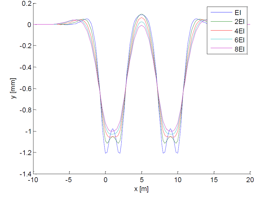
Virkning av økt bøyestivhet EI_x i skinnen.

Virkning av økt opplagringsstivhet k_d.

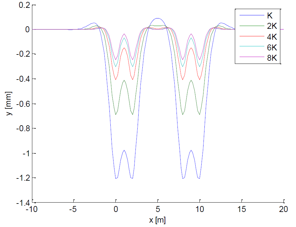
Figur 1.14 Virkning av skinne- og opplagringsstivhet på boggiindusert vertikal nedbøyning. Kurvene er kvalitative og skal ikke brukes som dimensjoneringsdiagram.(a) Virkning av økt bøyestivhet E I x i skinnen; og (b) Virkning av økt opplagringsstivhet k d.

1.5 Beregning av statiske spenninger: Eisenmanns metode

Eisenmanns metode [65, 68] gir lukkede ligninger for midlere spenninger og krefter i hvert lag av sporkonstruksjonen under en statisk hjullast \(Q\). Metoden bygger på Winklers bjelkemodell og er et vanlig analytisk verktøy for foreløpig spordimensjonering i europeisk praksis. Her presenteres metoden lag for lag.

Notasjonen som brukes i spenningsberegningene, er samlet i Tabell 1.3 før ligningene for de enkelte lagene innføres.

Symbol	Enhet	Betydning og beregningskonvensjon
\(P\)	kN eller t	Aksellast, det vil si den samlede lasten som bæres av begge hjulene på én aksel. Når lasten er angitt i tonn, må den omregnes til kraft før spenningsberegningene.
\(Q\)	N eller kN	Hjullast. I Eisenmann-ligningene med N og mm skal \(Q\) brukes i N.
\(Q_0\)	kN	Statisk hjullast uttrykt i kN for den forenklede formelen for kontaktspenning.
\(I_x\)	mm\(^4\)	Skinnens treghetsmoment om den horisontale nøytralaksen. Indeksen hindrer forveksling med manglende overhøyde.
\(D_c\)	mm	Manglende overhøyde brukt i drøftingen av kvasistatisk kurvelast.
\(a\)	mm	Senteravstand mellom svillene.
\(k_d\)	N/mm	Vertikal opplagringsstivhet for ett skinnesete (én halvsville). Praktiske verdier kan oppgis i kN/mm; multipliser med 1000 før bruk i ligninger med N og mm, som Ligning 1.7.
\(L\)	mm	Karakteristisk lengde for skinnebjelken på elastisk underlag.
\(F_0\)	N	Befestigelsens klemkraft ved ett skinnesete.
\(A_{rs}\), \(A_{sb}\)	mm\(^2\)	Effektive kontaktarealer mellom skinne–sville og sville–ballast. Verdier angitt i cm\(^2\) må multipliseres med 100.
\(t\), \(\varphi\)	–	Eisenmanns faktor for statistisk sikkerhet og sporkvalitetskoeffisient, brukt i DAF.

Tabell 1.3 Notasjon og beregningsenheter brukt i spenningsberegningene i dette kapitlet.

1.5.1 Skinnehode: kontaktspenning

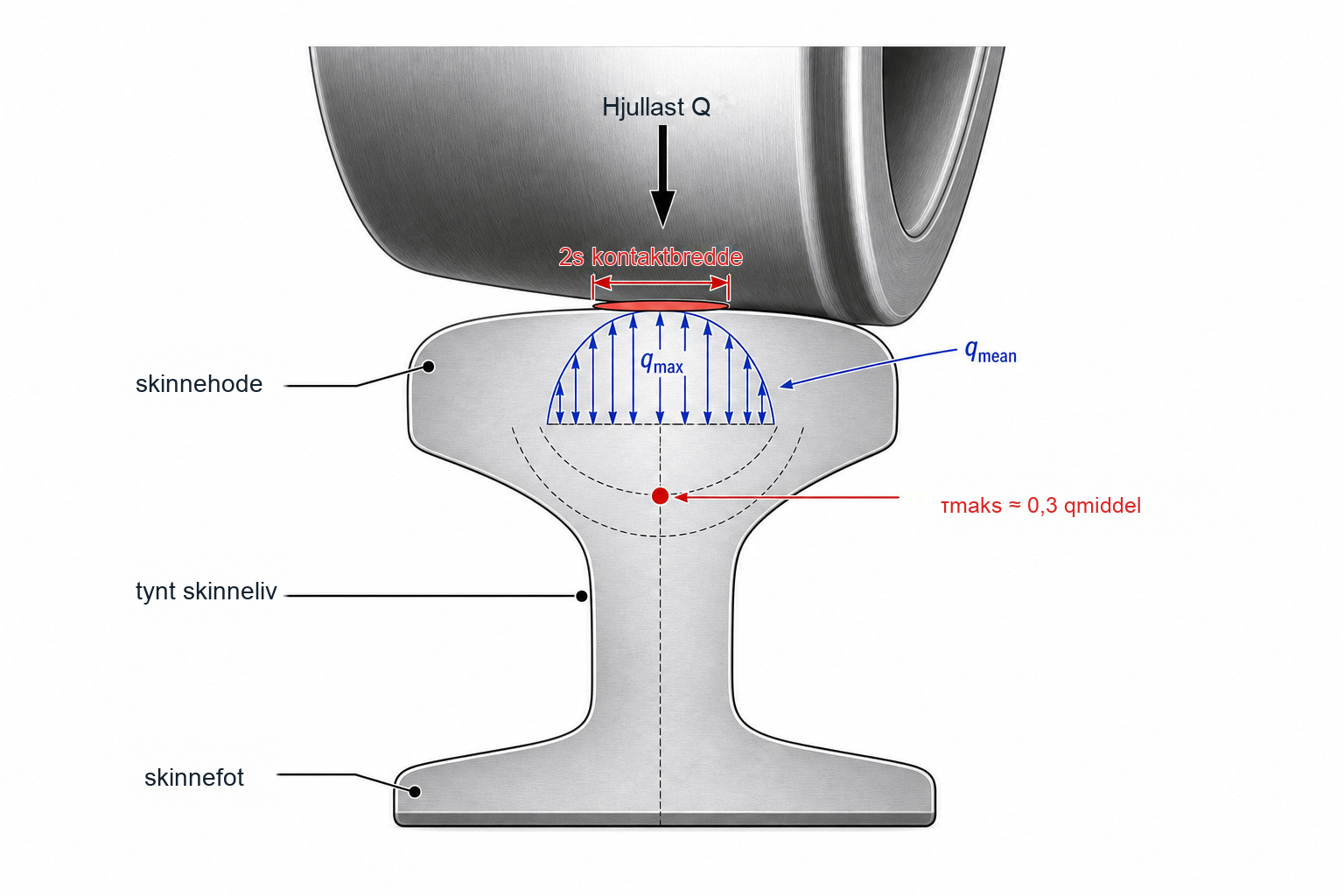
Den virkelige kontakten mellom hjul og skinne har en tredimensjonal, tilnærmet elliptisk trykkfordeling. For en innledende kontroll av skinnehodet erstatter Eisenmanns forenklede todimensjonale modell kontaktellipsen med en rektangulær stripe med bredde \(2s\) og benytter den midlere kontaktspenningen [64, 68, 15]:

\[ q_{\mathrm{mean}} = \sqrt{\frac{\pi E Q}{64(1-\nu^2)\,r\,s}} \]

(1.4)

der:

• \(Q\) = hjullast [N]

• \(E\) = elastisitetsmodul for skinnestål = 210 000 N/mm\(^2\)

• \(\nu\) = Poissons tall for stål = 0,30

• \(r\) = hjulradius [mm] (vanligvis 430–500 mm for nye hjul)

• \(s\) = antatt halv bredde av den rektangulære kontaktstripen mellom hjul og skinne [mm]

Med \(E=210\,000\) N/mm\(^2\), \(\nu=0{,}30\) og \(s=6\) mm blir Eisenmanns praktiske uttrykk [64, 68, 15]:

\[ q_{\mathrm{mean}} = 1374\sqrt{\frac{Q_0}{r}} \quad [\mathrm{N/mm^2}] \]

(1.5)

Her er \(Q_0\) den statiske eller kvasistatiske hjullasten i kN, mens \(r\) er hjulradiusen i mm. Koeffisienten 1374 er en enhetsavhengig koeffisient som omfatter forutsetningene ovenfor; den er ikke dimensjonsløs. For en gitt hjulradius gir denne forenklede linjekontaktmodellen \(q_{\mathrm{mean}}\propto\sqrt{Q_0}\). Modellen er forskjellig fra en full Hertz-løsning for den faktiske kontaktellipsen, der det største kontakttrykket skalerer med kubikkroten av normalkraften når geometri og materialegenskaper holdes konstante.

Den maksimale skjærspenningen oppstår under overflaten av skinnehodet og kan bidra til initiering av sprekker fra rullende kontaktutmattelse (RCF). I denne innledende kontrollen tilnærmes den som [68]:

\[ \tau_{\max} \approx 0{,}3\;q_{\mathrm{mean}} \]

(1.6)

i en dybde på omtrent 4–6 mm under kjøreflaten.

Ligning 1.6 er en tilnærming innenfor Eisenmanns forenklede linjekontaktmodell og brukes bare i den innledende kontrollrekken i dette kapitlet. Den skal ikke kombineres med trykkforholdene i en full Hertz-ellipse. I den tredimensjonale Hertz-modellen er det arealmidlede trykket \(\bar p=N/(\pi ab)\), mens det største trykket er \(p_0=3N/(2\pi ab)=1{,}5\bar p\). Ingen av disse størrelsene er identisk med Eisenmanns \(q_{\mathrm{mean}}\). Den største skjærspenningen under overflaten og dybden der den opptrer, avhenger også av kontaktellipsens akseforhold og friksjonsbelastningen. Rullende kontaktutmattelse introduseres fra et feilperspektiv i kapittel 4; den fullstendige kontaktmodellen utvikles senere i kapittel 10.

Spenningskonsentrasjonen i hjul–skinne-kontakten er vist skjematisk i Figur 1.15, inkludert kontaktbredden og plasseringen av den maksimale skjærspenningen under overflaten.

Figur 1.15 Skjematisk fordeling av kontaktspenninger etter Hertz’ teori i skinnehodet, med kontaktbredde 2s, kontakttrykk q og omtrentlig plassering av maksimal skjærspenning under overflaten.

1.5.2 Skinnefot: bøyespenning

Skinnen bøyes under den konsentrerte hjullasten i samsvar med Winkler-modellen. Den karakteristiske lengden \(L\) er den grunnleggende parameteren i løsningen for en bjelke på elastisk underlag [65]:

\[ L = \sqrt[4]{\frac{4\,E\,I_x\,a}{k_d}} \]

(1.7)

der:

• \(E\) = elastisitetsmodul for skinnestål [N/mm\(^2\)]

• \(I_x\) = treghetsmoment for skinnetverrsnittet om den horisontale nøytralaksen [mm\(^4\)]

• \(a\) = senteravstand mellom svillene [mm]

• \(k_d\) = vertikal opplagringsstivhet for ett skinnesete (én halvsville) [N/mm]

Den karakteristiske lengden \(L\) angir avstanden skinnen fordeler punktlasten over: En større \(L\) betyr at lasten fordeles over flere sviller. Det reduserer den største svillekraften, men reduserer ikke nødvendigvis bøyespenningen i skinnen. Typiske verdier av \(L\) for ballasterte hovedbanespor ligger mellom 700–1100 mm.

Den midlere strekkspenningen fra bøyning midt under skinnefoten, som er det kritiske snittet for utmatting, er [65, 68]:

\[ \sigma_{\mathrm{mean}} = \frac{Q \cdot L}{4\,W_{yf}} \]

(1.8)

der \(W_{yf}\) [mm\(^3\)] er motstandsmomentet for skinnetverrsnittet med hensyn til den nederste fiberen (skinnefoten).

Tabell 1.4 viser de geometriske egenskapene til de to skinneprofilene som er mest brukt i Norge. Profil 60E1 (tidligere betegnet UIC 60) er standard ved nybygging på hovedbaner; UIC 54 finnes på eldre strekninger og sidebaner.

Profil	\(A\) [cm\(^2\)]	\(I_x\) [cm\(^4\)]	\(W_{yf}\) [cm\(^3\)]	\(W_{yh}\) [cm\(^3\)]	Masse [kg/m]
UIC 54	69,34	2 346	235	268	54,43
60E1 (UIC 60)	76,86	3 055	335	378	60,34

Tabell 1.4 Geometriske egenskaper for skinneprofiler som brukes i Norge (Bane NORs tekniske regelverk, Overbygning/Prosjektering/Sporkonstruksjoner [10]).

1.5.3 Sville: støttepunktkraft og kontaktspenning

Den midlere vertikale kraften på den mest belastede svillen under ett hjul beregnes på grunnlag av skinnens belastede lengde [68]:

\[ F_{\mathrm{mean}} \approx \frac{Q \cdot a}{2\,L} \]

(1.9)

der \(a\) er svilleavstanden, og \(2L\) er den effektive lastfordelingslengden. Opplagringsstivheten \(k_d\) styrer den karakteristiske lengden \(L\) i Winkler-modellen, men skal ikke multipliseres direkte inn i dette kraftuttrykket.

Det midlere kontakttrykket i grensesnittet mellom skinne og sville (eller kontakttrykket ved skinnesetet) må ta hensyn til forspenningen fra befestigelsens klemkraft \(F_0\):

\[ \sigma_{rs} = \frac{F_0 + F_{\mathrm{mean}}}{A_{rs}} \]

(1.10)

der:

• \(F_0\) = samlet klemkraft fra befestigelsen ved skinnesetet [N] (begge klemfjærene, én skinne)

• \(A_{rs}\) = effektiv kontaktflate ved skinnesetet [mm\(^2\)] (med underlagsplate: platens areal; uten underlagsplate: skinnefotens areal)

De tillatte kontakttrykkene mellom skinne og sville i henhold til Bane NORs tekniske regelverk [10] er:

• Sviller av bartre (furu): \(\sigma_{rs} \leq 1{,}0\)–\(1{,}5\) N/mm\(^2\)

• Sviller av løvtre (eik): \(\sigma_{rs} \leq 1{,}5\)–\(2{,}5\) N/mm\(^2\)

• Forspente betongsviller: \(\sigma_{rs} \leq 4{,}0\) N/mm\(^2\)

Betongsviller er standard på norske hovedbaner; tresviller er beholdt på enkelte lite trafikkerte sidebaner og sidespor [130].

1.5.4 Ballast: kontaktspenning mellom sville og ballast

Lasten fordeles fra svillen til ballasten over det effektive bærearealet \(A_{sb}\) under én halvsville. Den midlere kontaktspenningen mellom sville og ballast er [68, 128]:

\[ \sigma_{sb} = \frac{F_{\mathrm{mean}}}{A_{sb}} \]

(1.11)

Det tillatte kontakttrykket mot ballasten i Bane NORs tekniske regelverk [10] er:

\[ \sigma_{sb} \leq 0{,}50\ \mathrm{N/mm^2} \]

(1.12)

Denne grensen bestemmer det minste nødvendige bærearealet \(A_{sb}\) for en gitt last og sporstivhet. Ligning 1.11 viser at \(\sigma_{sb}\) kan reduseres ved å:

• Øke \(A_{sb}\): bruke bredere eller lengre betongsviller (f.eks. toblokksviller i stedet for monoblokksviller, eller type B70 i stedet for B60).

• Redusere \(F_{\mathrm{mean}}\): redusere svilleavstanden \(a\) eller øke den karakteristiske lengden \(L\) (for eksempel ved å øke skinnens bøyestivhet eller redusere opplagringsstivheten, forutsatt at grensene for nedbøyning og setning fortsatt er oppfylt).

Oppsett for regneeksempel.

Et konvensjonelt hovedbanespor kontrolleres mot spenningsgrensene i Bane NORs tekniske regelverk ved \(v = 120\) km/h. Følgende data brukes i den statiske beregningen nedenfor og i den senere dynamiske fortsettelsen.

Parameter	Verdi
Statisk hjullast	\(Q = 100\ \mathrm{kN}\)
Skinneprofil	UIC 54: \(I_x = 2346\times10^4\ \mathrm{mm^4}\), \(W_{yf} = 235\times10^3\ \mathrm{mm^3}\), \(r = 500\ \mathrm{mm}\)
Vertikal opplagringsstivhet, ett skinnesete	\(k_d = 12\ \mathrm{kN/mm}=12\,000\ \mathrm{N/mm}\)
Svilleavstand	\(a = 600\ \mathrm{mm}\)
Befestigelsens klemkraft	\(F_0 = 20\ \mathrm{kN}\) (per skinne, per skinnesete)
Kontaktflate mellom skinne og sville	\(A_{rs} = 550\ \mathrm{cm^2}\) (betongsville med underlagsplate)
Kontaktflate mellom sville og ballast	\(A_{sb} = 837\ \mathrm{cm^2}\) (bæreareal under en halvsville)
Materiale	\(E = 210\,000\ \mathrm{N/mm^2}\), \(\nu = 0{,}3\)
Sporkvalitet	Normal (\(\varphi = 0{,}2\))

Regneeksempel: kontroll av statiske spenninger.

Med dataene fra oppsettet for regneeksemplet blir den statiske kontaktspenningen mellom hjul og skinne

\[ \begin{aligned} q_{\mathrm{mean}} &= 1374\sqrt{\frac{Q_0}{r}},\\ &= 1374\sqrt{\frac{100}{500}},\\ &= 614{,}5\ \mathrm{N/mm^2}. \end{aligned} \]

og den omtrentlige maksimale skjærspenningen under overflaten blir \(\tau_{\max}\approx0{,}3q_{\mathrm{mean}}=184{,}3\) N/mm\(^2\).

Den karakteristiske lengden er

\[ L = \sqrt[4]{\frac{4 \times 210\,000 \times 2346\times10^4 \times 600}{12\,000}} = 996\ \mathrm{mm}. \]

Bøyespenningen i skinnefoten og kraften på den mest belastede svillen er

\[ \begin{aligned} \sigma_{\mathrm{mean}} &= \frac{100\,000 \times 996}{4 \times 235\,000} = 105{,}9\ \mathrm{N/mm^2},\\ F_{\mathrm{mean}} &= \frac{100\,000 \times 600}{2 \times 996} = 30{,}1\ \mathrm{kN}. \end{aligned} \]

Kontaktspenningene i grensesnittene blir deretter

\[ \sigma_{rs} = \frac{20\,000 + 30\,100}{550 \times 100} = 0{,}91\ \mathrm{N/mm^2} \leq 4{,}0\ \mathrm{N/mm^2}, \]

\[ \sigma_{sb} = \frac{30\,100}{837 \times 100} = 0{,}360\ \mathrm{N/mm^2} \leq 0{,}50\ \mathrm{N/mm^2}. \]

Begge de statiske kontrollene av grensesnittene ligger innenfor grensene i Bane NORs tekniske regelverk.

1.6 Dynamiske effekter av trafikklaster

Statisk aksellast er bare utgangspunktet for dimensjonering av sporet. Hastighet, kurvatur, vind og ujevnheter i sporet gir dynamiske virkninger som kan være dimensjonerende for lokale spenninger og vedlikeholdsbehov.

1.6.1 Kvasistatiske krefter: kurver og sidevind

Når et tog kjører gjennom en horisontalkurve med hastighet \(v\) [km/h] og radius \(R\) [m], virker sentrifugalakselerasjonen utover på både kjøretøyet og innholdet. Hvis sporet har en overhøyde \(h_a\) [mm], blir sentrifugalvirkningen delvis balansert. Den manglende overhøyden \(D_c\) [mm] angir den ubalanserte sentrifugalvirkningen [68]:

\[ \begin{aligned} D_c &= h_{\mathrm{ideal}} - h_a,\\ h_{\mathrm{ideal}} &= \frac{11{,}8\,v^2}{R}\ \text{[mm]}. \end{aligned} \]

(1.13)

Manglende overhøyde gir først en ubalansert sideveis treghetskraft. Denne kraften skaper deretter et rullemoment om kontaktlinjen mellom hjul og skinne, slik at den vertikale hjullasten på ytterskinnen øker og hjullasten på innerskinnen reduseres. Et dimensjonsriktig estimat er:

\[ Y_c = G\,\frac{D_c}{b_c} \]

(1.14)

\[ \Delta Q = \frac{Y_c h_d + Y_w h_w}{b_g} \]

(1.15)

der \(Y_c\) = kurveindusert sideveis treghetskraft per aksel [kN], \(G\) = akseltyngde [kN], \(D_c\) = manglende overhøyde [mm], \(b_c\) = effektiv overhøydebasis (omtrent 1500 mm), \(\Delta Q\) = økning i vertikal hjullast på ytterskinnen [kN], \(Y_w\) = sidevindkraft per aksel [kN], \(h_d\) = høyden til tyngdepunktet over skinnen [m], \(h_w\) = høyden til vindkraftens resultant over skinnen [m], og \(b_g\) = sideveis avstand mellom kontaktpunktene mellom hjul og skinne [m]. Dermed:

\[ \begin{aligned} Q_{\mathrm{outer}} &\approx \frac{G}{2} + \Delta Q,\\ Q_{\mathrm{inner}} &\approx \frac{G}{2} - \Delta Q. \end{aligned} \]

(1.16)

Sentrifugalbidraget til hjullasten på ytterskinnen utgjør typisk 10–25% av den statiske hjullasten, avhengig av hastighet, manglende overhøyde, høyden til kjøretøyets tyngdepunkt og sporviddegeometrien.

1.6.2 Ujevnheter i sporet og kjøretøyfeil

I praksis er sporgeometrien aldri helt jevn. Geometriske ujevnheter, blant annet skinnerifler, skinneskjøter, overgangssoner og sporveksler, samt kjøretøyfeil som hjulslagflater og urunde hjul, gir alle tilleggskrefter utover den statiske verdien [130, 91]. Slike lokale feil kan gjøre en ellers jevn hjulpassering til en slaglignende belastning.

Figur 1.16 Feil som kan forsterke dynamiske hjullaster: (a) hjulslagflate eller løpebaneskade; (b) skinnerifler; og (c) en squat eller annen lokal feil i skinnehodet.

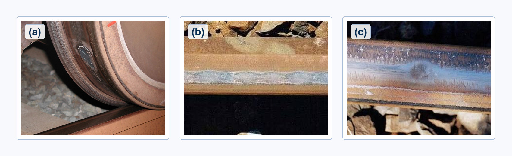
Dynamiske krefter er i sin natur stokastiske: De varierer fra én akselpassering til den neste, avhenger av den konkrete kombinasjonen av spor- og kjøretøytilstand og kan ikke forutsies deterministisk [117]. Derfor benyttes en probabilistisk dimensjoneringsmetode, uttrykt ved en dynamisk forsterkningsfaktor (Dynamic Amplification Factor, DAF).

1.6.3 Dynamisk forsterkningsfaktor (DAF)

Eisenmanns DAF [65, 68] forsterker de statiske spenningene og kreftene for å gi de dimensjonerende (maksimalt forventede) verdiene. Den er definert som:

\[ \mathrm{DAF} = 1 + t\,\varphi \qquad \text{for } v < 60\ \mathrm{km/h} \]

(1.17)

\[ \mathrm{DAF} = 1 + t\,\varphi\!\left(1 + \frac{v - 60}{140}\right) \qquad \text{for } 60 \leq v \leq 200\ \mathrm{km/h} \]

(1.18)

der:

• \(v\) = toghastighet [km/h]

• \(\varphi\) = sporkvalitetskoeffisient (se Tabell 1.5)

• \(t\) = faktor for statistisk sikkerhet, lik antall standardavvik over middelverdien (Tabell 1.5)

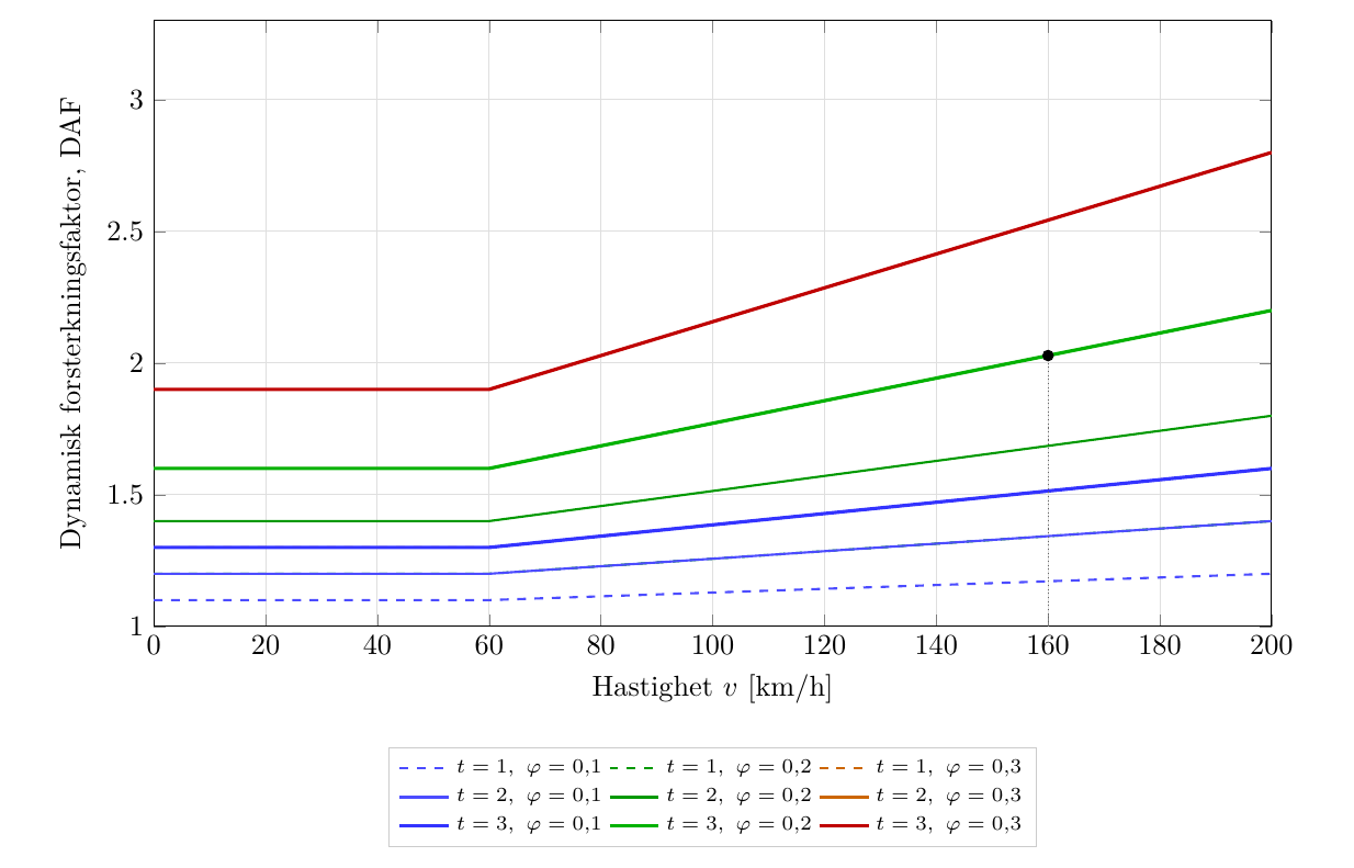
Det statistiske grunnlaget for DAF er viktig å forstå. Aksellasten øker ikke fordi kjøretøyet blir tyngre; i stedet varierer den målte hjulkraften rundt den statiske verdien når kjøretøy og spor samvirker dynamisk. Det dynamiske lasttillegget antas å være normalfordelt med middelverdi lik null og standardavvik \(\varphi \cdot Q_{\mathrm{static}} \cdot (1 + (v-60)/140)\). Ved å velge \(t = 1, 2, 3\) velger den prosjekterende henholdsvis den 84., 97,7. eller 99,87. persentilen i lastfordelingen. For bøyespenninger i skinnen, befestigelser og opplagringer er \(t = 3\) standard. For ballast og undergrunn anses \(t = 2\) som tilstrekkelig [68].

Sporkvalitet	Beskrivelse	\(\boldsymbol{\varphi}\)	Anbefalt bruk
God	Nytt eller godt vedlikeholdt spor; regelmessig pakking	0,1	Høyhastighetsbaner
Normal	Standard vedlikeholdssyklus	0,2	Hovedbaner med blandet trafikk
Dårlig	Utsatt vedlikehold; høy feilutbredelse	0,3	Konservativ dimensjonering

Tabell 1.5 Sporkvalitetskoeffisient \(\varphi\) og faktor for statistisk sikkerhet \(t\) (Eisenmanns DAF-formel [65, 68]). Faktorer for statistisk sikkerhet: \(t = 3\) for bøyespenninger i skinnen, befestigelser og opplagringer (99,87. persentil); \(t = 2\) for ballast og undergrunn (97,7. persentil).

Hastighetsavhengigheten er vist i Figur 1.17 for tre sporkvalitetsklasser og tre nivåer for statistisk sikkerhet. Ved 160 km/h med normal sporkvalitet (\(\varphi = 0{,}2\)) og \(t = 3\):

\[ \mathrm{DAF} = 1 + 3\times0{,}2\times\!\left(1+\frac{160-60}{140}\right) = 1 + 0{,}6\times1{,}714 = 2{,}03. \]

Figur 1.17 Eisenmanns DAF for φ ∈ {0, 1, 0, 2, 0, 3} og t ∈ {1, 2, 3}. Den svarte markøren viser eksempelet med v = 160 km/h, normal sporkvalitet og DAF = 2, 03.

1.6.4 Dimensjonerende spenninger med DAF

De største (karakteristiske) spenningene og kreftene i kontrollene av sporkomponentene nedenfor beregnes ved å anvende riktig DAF på den statiske hjullasten. For størrelser som er lineære med hjullasten, tilsvarer dette å multiplisere den statiske verdien med DAF.

Den lokale kontrollen av skinnehodet behandles separat. Det fullstendige forenklede uttrykket er \(q_{\mathrm{mean}}=1374\sqrt{Q_0/r}\); kvadratroten omfatter hele forholdet \(Q_0/r\). For en gitt hjulradius er kontaktspenningen proporsjonal med kvadratroten av hjullasten, men i det praktiske Eisenmann-uttrykket benyttes statisk eller kvasistatisk hjulkraft. DAF med \(t=3\) for sporkomponenter skal derfor ikke automatisk settes inn i denne formelen  [68, 15]. En dynamisk analyse av hjul–skinne-kontakten må i stedet ta utgangspunkt i en dynamisk hjulkraft som er bestemt separat, og en egnet kontaktmodell.

Tabell 1.6 skiller derfor mellom den separate kontrollen av skinnehodet og de DAF-forsterkede responsene i sporkomponentene.

Komponent / grenseflate	Statisk verdi	Dynamisk dimensjonerende verdi	Typisk kontroll
Kontakt mellom hjul og skinne	\(q_{\mathrm{mean}} = 1374\sqrt{Q_0/r}\)	Separat kontaktanalyse; DAF anvendes ikke her	Kan bidra til utmatting i skinnehodet og risiko for RCF
Bøyning av skinnefoten	\(\sigma_{\mathrm{mean}} = QL/(4W_{yf})\)	\(\sigma_d = \mathrm{DAF}_{t=3}\,\sigma_{\mathrm{mean}}\)	Strekkspenning i skinnefoten; margin mot utmatting / brudd
Støttepunktkraft ved skinnesetet	\(F_{\mathrm{mean}} \approx Qa/(2L)\)	\(F_d = \mathrm{DAF}_{t=3}\,F_{\mathrm{mean}}\)	Belastning på mellomlegg, befestigelse og sville ved skinnesetet
Trykk mellom skinne og sville	\(\sigma_{rs}=(F_0+F_{\mathrm{mean}})/A_{rs}\)	\(\sigma_{rs,d}=(F_0+F_d)/A_{rs}\)	\(\leq 4{,}0\) N/mm\(^2\) for betongsviller
Trykk mellom sville og ballast	\(\sigma_{sb}=F_{\mathrm{mean}}/A_{sb}\)	\(\sigma_{sb,d}=\mathrm{DAF}_{t=2}\,\sigma_{sb}\)	\(\leq 0{,}50\) N/mm\(^2\) i ballastkontakten
Toppen av undergrunnen	Beregnet ut fra lastspredning gjennom ballast/forsterkningslag	Bruk \(\mathrm{DAF}_{t=2}\) på den overførte vertikalspenningen	Sammenlign med undergrunnens bæreevne og setningskriterier

Tabell 1.6 Sammendrag av den separate kontrollen av skinnehodet og de DAF-baserte beregningene for sporkomponentene (basert på [64, 65, 68, 15]).

Regneeksempel: dynamiske dimensjonerende verdier.

For normal sporkvalitet er \(\varphi=0{,}2\). Selv om dimensjonerende hastighet er 120 km/h, vises også lavhastighetstilfellet \(v=20\) km/h for å gjøre DAF-multiplikasjonen tydelig:

\[ \begin{aligned} \mathrm{DAF}_{t=3}(20) &= 1 + 3\times0{,}2 = 1{,}60,\\ \mathrm{DAF}_{t=2}(20) &= 1 + 2\times0{,}2 = 1{,}40. \end{aligned} \]

Ved \(v=120\) km/h,

\[ \mathrm{DAF}_{t=3}(120) = 1 + 3\times0{,}2\times\!\left(1+\frac{120-60}{140}\right) = 1{,}857, \]

\[ \mathrm{DAF}_{t=2}(120) = 1 + 2\times0{,}2\times\!\left(1+\frac{120-60}{140}\right) = 1{,}571. \]

Den forenklede kontrollen av skinnehodet beholdes som den separate statiske eller kvasistatiske verdien \(q_{\mathrm{mean}}=614{,}5\) N/mm\(^2\), beregnet ovenfor. Verdien forsterkes ikke på nytt med DAF for sporkomponenter i dette eksempelet. Dersom det kreves en dynamisk kontaktanalyse, må den dynamiske hjulkraften bestemmes separat før en egnet kontaktmodell anvendes. Bøyespenningen i skinnefoten er lineær med hjullasten og multipliseres derfor direkte med \(\mathrm{DAF}_{t=3}\):

\[ \begin{aligned} \sigma_d(20) &= 1{,}60\times105{,}9 = 169{,}4\ \mathrm{N/mm^2},\\ \sigma_d(120) &= 1{,}857\times105{,}9 = 196{,}7\ \mathrm{N/mm^2}. \end{aligned} \]

For grenseflaten mellom skinne og sville er det bare \(F_{\mathrm{mean}}\) som forsterkes; befestigelsens klemkraft \(F_0\) forblir statisk:

\[ \begin{aligned} \sigma_{rs,d}(20) &= \frac{20\,000 + 48\,200}{550\times100} = 1{,}24\ \mathrm{N/mm^2},\\ \sigma_{rs,d}(120) &= \frac{20\,000 + 55\,900}{550\times100} = 1{,}38\ \mathrm{N/mm^2}. \end{aligned} \]

For grenseflaten mellom sville og ballast benyttes \(\mathrm{DAF}_{t=2}\) i ballastkontrollen:

\[ \begin{aligned} \sigma_{sb,d}(20) &= 1{,}40\times0{,}360 = 0{,}504\ \mathrm{N/mm^2},\\ \sigma_{sb,d}(120) &= 1{,}571\times0{,}360 \approx 0{,}565\ \mathrm{N/mm^2}. \end{aligned} \]

Størrelse	Statisk	\(v = 20\) km/h \((t=3:\ 1{,}60;\ t=2:\ 1{,}40)\)	\(v = 120\) km/h \((t=3:\ 1{,}86;\ t=2:\ 1{,}57)\)	Grense
Kontaktspenning i skinnehodet \(q\) [N/mm\(^2\)]	614,5	–	–	Separat kontroll
Bøyespenning i skinnefoten \(\sigma\) [N/mm\(^2\)]	105,9	169,4	196,7	Ikke relevant
Trykk mellom skinne og sville \(\sigma_{rs}\) [N/mm\(^2\)]	0,91	1,24	1,38	\(\leq 4{,}0\)
Trykk mellom sville og ballast \(\sigma_{sb}\) [N/mm\(^2\)]	0,360	0,504	0,565	\(\leq 0{,}50\)

Tabell 1.7 Separat statisk kontaktkontroll og DAF-forsterkede verdier for sporkomponentene i regneeksempelet.

Trykket mellom sville og ballast overskrider grensen på \(0{,}50\) N/mm\(^2\) marginalt allerede ved 20 km/h (\(0{,}504\) N/mm\(^2\)) og mer tydelig ved 120 km/h. Ballastgrenseflaten er derfor dimensjonerende i dette eksempelet. Ved 120 km/h er nødvendig bæreareal for en halvsville omtrent 947 cm\(^2\) dersom alle andre forutsetninger er uendret. Marginen kan forbedres ved å øke svillens bæreareal, redusere svilleavstanden og beregne \(L\) og \(F_{\mathrm{mean}}\) på nytt, eller stille strengere krav til sporkvaliteten.

1.7 Kontroll av skinnespenninger for hjulgrupper

Eisenmann-beregningene ovenfor tar utgangspunkt i hjullasten og den mest belastede svillen ved innledende spenningskontroller. For kjøretøy med boggier kan nabohjul på samme skinne også påvirke bøyemomentet under et referansehjul. En kompakt påvirkningslinjekontroll etter Winkler–Zimmermann er nyttig når en kontroll av spenningen i skinnefoten må ta eksplisitt hensyn til akselavstanden [68, 62, 65].

For et hjul i avstanden \(x\) fra referansehjulet er påvirkningskoeffisienten

\[ \begin{aligned} \xi &= \frac{x}{L},\\ \mu &= e^{-\xi}(\cos\xi - \sin\xi). \end{aligned} \]

(1.19)

der \(L\) er skinnens karakteristiske lengde på opplagringen. For referansehjulet er \(x=0\) og \(\mu=1\). La \(N_\mathrm{w}\) være antall hjul på samme skinne som inngår i kontrollen. Hjulgruppefaktoren defineres som

\[ S_\mu = \sum_{i=1}^{N_\mathrm{w}} \mu_i. \]

Når den dimensjonerende dynamiske hjullasten er valgt, kan det største bøyemomentet i skinnen skrives som

\[ M_\mathrm{max} = \frac{Q_\mathrm{design} L}{4}S_\mu, \]

(1.20)

der \(Q_\mathrm{design}\) er dimensjonerende hjullast på én skinne, og \(L\) settes inn i meter når \(M_\mathrm{max}\) skal angis i kNm. Tilsvarende strekkspenning i skinnefoten er

\[ \sigma_\mathrm{foot} = \frac{M_\mathrm{max}\,[\mathrm{kNm}]\cdot10^6}{W_{yf}\,[\mathrm{mm}^3]} \quad [\mathrm{N/mm^2}]. \]

(1.21)

De følgende korte eksemplene viser hvordan påvirkningskoeffisientene brukes i praksis.

Regneeksempel: toakslet boggi.

Anta en innledende skinnekontroll med karakteristisk lengde \(L=0{,}80\) m, dimensjonerende hjullast \(Q_\mathrm{design}=140\) kN, motstandsmoment for skinnefoten \(W_{yf}=335\cdot10^3\) mm\(^3\) og et annet hjul på samme skinne med akselavstand \(x=2{,}0\) m. Referansehjulet har \(\mu_1=1\). For det andre hjulet,

\[ \begin{aligned} \xi_2&=\frac{x}{L}=\frac{2{,}0}{0{,}80}=2{,}50,\\ \mu_2&=e^{-2{,}50}(\cos 2{,}50-\sin 2{,}50)=-0{,}115. \end{aligned} \]

Dermed

\[ S_\mu = \sum_{i=1}^{2}\mu_i = \mu_1+\mu_2 = 1-0{,}115 = 0{,}885. \]

Det største bøyemomentet og spenningen i skinnefoten blir da

\[ M_\mathrm{max} =\frac{140\cdot0{,}80}{4}\cdot0{,}885 =24{,}8\,\mathrm{kNm}, \]

\[ \sigma_\mathrm{foot} =\frac{24{,}8\cdot10^6}{335\cdot10^3} =74\,\mathrm{N/mm^2}. \]

I dette eksempelet ligger nabohjulet i en negativ del av påvirkningslinjen, og det reduserer derfor bøyemomentet ved referansehjulet noe. Dette er mulig fordi skinnen oppfører seg som en bjelke på elastisk underlag, ikke som en fritt opplagt bjelke.

Rask sensitivitetskontroll: et nærmere nabohjul.

Hvis det samme nabohjulet lå betydelig nærmere, for eksempel \(x=0{,}40\) m med samme \(L=0{,}80\) m, ville

\[ \begin{aligned} \xi_2&=0{,}50,\\ \mu_2&=e^{-0{,}50}(\cos0{,}50-\sin0{,}50)=0{,}241, \end{aligned} \]

slik at

\[ S_\mu=\sum_{i=1}^{2}\mu_i=1+0{,}241=1{,}241. \]

Den samme dimensjonerende hjullasten ville gitt

\[ \begin{aligned} M_\mathrm{max} &=\frac{140\cdot0{,}80}{4}\cdot1{,}241 =34{,}8\,\mathrm{kNm},\\ \sigma_\mathrm{foot} &=104\,\mathrm{N/mm^2}. \end{aligned} \]

Avstanden i forhold til \(L\) er derfor avgjørende: Nabohjul skal ikke uten videre legges til som fulle hjullaster.

Denne kontrollen erstatter ikke den lagvise Eisenmann-metoden ovenfor. Den er en supplerende kontroll av skinnebøyning for tilfeller der avstanden mellom nabohjul og skinneprofilets egenskaper må angis eksplisitt.

1.7.1 Klassiske parametere for kontinuerlig understøttelse

I eldre norsk og tysk dimensjoneringspraksis beskrives skinneopplagringen ikke ved en diskret stivhet ved skinnesetet \(k_d\) og svilleavstand \(a\), men ved en ballastkoeffisient \(C_b\) (N/cm\(^3\)) som virker over en ekvivalent bredde for en kontinuerlig understøttet skinne \(b\). De to beskrivelsene kan omregnes til hverandre: Den kontinuerlige fundamentstivheten per lengdeenhet er \(C_b\,b\), og den karakteristiske lengden blir

\[ L=\sqrt[4]{\frac{4\,E\,I_x}{b\,C_b}}, \]

(1.22)

som erstatter den diskrete formen i ligning 1.7 når \(C_b\) og \(b\) er de oppgitte opplagringsdataene. Tre ytterligere konvensjoner hører til denne klassiske metoden og brukes når eldre datasett eller klassiske dimensjoneringstilfeller er formulert etter den:

• Korreksjon for hjulkraftforskyvning. Et tillegg på \(0{,}1\,Q_\mathrm{static}\) legges til den statiske hjulkraften før skinnekontrollen. Tillegget representerer lastoverføring mellom hjulene på en aksel som følge av overhøyde, kurvekjøring og lastens eksentrisitet.

• Klassisk hastighetsfaktor. Den dimensjonerende dynamiske hjullasten skrives \(Q_\mathrm{design}=Q\,(1+n\,\varphi_v)\), der hastighetsfaktoren er \(\varphi_v = 1 + 0{,}5\,(v-60)/80\) for \(60<v\leq140\) km/h (og \(\varphi_v=1\) under 60 km/h), mens \(n\) beskriver sportilstanden: \(n=0{,}1\) for svært god, \(n=0{,}2\) for god og \(n=0{,}25\) for annen eller middels sportilstand. Merk nøye at hastighetsfaktoren \(\varphi_v\) ikke er den samme størrelsen som Eisenmanns sporkvalitetskoeffisient \(\varphi\) som ble brukt tidligere i dette kapitlet; senket indeks \(v\) brukes her for å skille de to symbolene.

• Minste hjulradius og tilhørende diameter. Det klassiske hjulstørrelseskriteriet begrenser kontaktspenningen ved en gitt hjulkraft ved å kreve minsteverdien for radius som defineres rett nedenfor.

Minste hjulradius er

\[ r_\mathrm{min}=1{,}67\cdot10^{6}\,Q\left(\frac{\nu_s}{\sigma_\mathrm{break}}\right)^{2}, \]

(1.23)

der \(Q\) er i kN, skinnens strekkfasthet \(\sigma_\mathrm{break}\) er i N/mm\(^2\), \(r_\mathrm{min}\) er i mm og \(\nu_s\) er en utnyttelsesfaktor for hjullasten som avhenger av banekategorien (\(\nu_s = 1{,}2\) er en representativ verdi for en godsbane av andre orden). Den tilhørende minste hjuldiameteren er \(D_\mathrm{min}=2r_\mathrm{min}\); en oppgitt hjuldiameter \(D\) skal sammenlignes med \(D_\mathrm{min}\), ikke direkte med \(r_\mathrm{min}\). Disse konvensjonene gjør det mulig å tolke klassiske opplagringsbeskrivelser konsekvent ved omregning mellom linjelastdata og diskret opplagringsstivhet ved ett skinnesete (én halvsville).

1.8 Bane NORs overbygningsklasser

Bane NOR klassifiserer sporet i overbygningsklasser (hver klasse betegnes som en overbygningsklasse) som angir største tillatte aksellast som funksjon av hastigheten [32, 169]. Hver banestrekning tildeles en overbygningsklasse basert på skinneprofil, svilletype og svilleavstand, ballasttykkelse og tilstanden i undergrunnen. Klassen er et viktig grunnlag for å avgjøre hvilke kjøretøy som kan tillates på strekningen, men driften kan også være begrenset av bruer, tilstanden i underbygningen, sporgeometri, lokale hastighetsbegrensninger og kjøretøyspesifikke godkjenninger.

Den kompakte klasseoversikten i Tabell 1.8 knytter disse infrastrukturklassene til grensene for aksellast og hastighet som brukes senere i kompendiet. Verdiene er hentet fra Bane NORs Operativt regelverk, SJN 2.18.1, oppdatert 15. august 2025 [32].

Klasse	Personvogner		Motorvognsett (EMU/DMU)
	Aksellast [t]	v [km/h]	Aksellast [t]	v [km/h]
a	16	90	16	90
b	18	100	18	100
c	18	160	20,5/18	130/160
c+	18	160	20,5	160
d	18	230	20,5/20/18/17	160/200/250/300
Ofotbanen	18	130	20,5	130

Klasse	Gods- og arbeidskjøretøy
	Aksellast [t]	v [km/h]	vboggi [km/h]
a	22,5/16,5	30/70	30/70
b	22,5/20,5/18	30/70/80	30/70/80
c	22,5/20,5/18	80/90/100	90/100/110
c+	241/22,5/20,5/18	50/90/100/110	50/100/110/120
d	25/22,5/18	70/100/110	70/120/120
Ofotbanen	31/22,5	50/702	50/70

Tabell 1.8 Bane NORs overbygningsklasser fra Operativt regelverk/SJN 2.18.1 (oppdatert 15. august 2025) [32]. Det er nødvendig med separate grenser fordi personvogner, motorvognsett og gods-/arbeidskjøretøy har ulik akselavstand og dynamisk oppførsel.

¹Verdien 24 t gjelder bare på Nordlandsbanen mellom Guldsmedvik (km 499,517) og Ørtfjell (km 534,630). ²Største hastighet for tomme malmvogner er 60 km/h.

I tabellen for gods- og arbeidskjøretøy er \(v_\mathrm{boggi}\) største hastighet for boggikjøretøy som er godkjent etter EN 14363. Skråstrekseparerte aksellaster og hastigheter hører sammen etter posisjon i hver rad; den første aksellasten hører for eksempel sammen med den første hastigheten. Verdien 24 t i klasse c+ gjelder bare Nordlandsbanen, Guldsmedvik–Ørtfjell. På Ofotbanen er tomme malmvogner begrenset til 60 km/h selv om tabellen viser 70 km/h for den tilhørende klasseverdien. Raden for Ofotbanen skal leses som en strekningstilpasset klassetabell, ikke som en generell tillatelse for alle kjøretøy. Malmtog kjører vanligvis med 30 t aksellast, mens 31 t er grensen for infrastrukturen/særreglene som vises i klassetabellen. Bruk av denne grensen er fortsatt avhengig av gjeldende Network Statement, kjøretøygodkjenning, begrensninger i bruer og underbygning samt lokale hastighetsforhold [30, 10].

Når det gjelder skinnekvalitet, krever Bane NORs tekniske regelverk [10] høyfaste, hodeherdede eller premiumkvaliteter for baner med høy aksellast:

• For aksellaster \(\leq 22{,}5\) t: Kvalitet R260 (minste strekkfasthet 880 N/mm\(^2\)) er standard.

• For aksellaster \(> 24\) t: Bane NOR angir premiumkvaliteter som R350HT, R370CrHT, R400HT eller R400 UHC XR, uavhengig av kurveradius.

• Kvalitet R200 (minst 680 N/mm\(^2\)) er bare tillatt på baner med lav hastighet og liten trafikk.

Valget av skinneprofil er knyttet til overbygningsklassen: 60E1 er standard for klassene c, c+ og d; UIC 54 kan brukes for klassene a og b [85]. Ofotbanens drift med høy aksellast krever skinnestål av premiumkvalitet og strekningstilpasset godkjenning. Tillatt aksellast i drift må overholde begrensninger i underbygning, bruer og geometri i tillegg til overbygningsklassen [165, 10].

1.9 Oppsummering

Trafikkbehov. Lastene som virker på sporet, bestemmes først av jernbanetjenesten: bybaner, konvensjonelle baner med blandet trafikk, korridorer for tung godstrafikk og spesialiserte jernbaner stiller ulike krav til aksellast, hastighet, bremsing, akselerasjon og gjentatte trafikkbelastninger. Kjøretøybetegnelser som Bo'Bo' og Co'Co' beskriver derfor kjøretøyet og viser ingeniøren hvordan vekten og trekkreftene fordeles mellom aksler og boggier.

Lastoverføring. En vertikal hjullast starter som en konsentrert kontaktkraft i skinnehodet, men spres gradvis gjennom skinne, sville, ballast, forsterkningslag og formasjonsplan. Spenningene avtar med dybden fordi det belastede arealet øker, men dette betyr ikke at de nedre lagene er uviktige. Svak ballast eller et svakt formasjonsplan endrer opplagringsstivheten og kan øke skinnebøyning, svilletrykk og langsiktige setninger.

Dynamiske virkninger. Statisk aksellast og hjullast gir de grunnleggende dimensjoneringsstørrelsene, men den reelle trafikklasten omfatter kvasistatiske krefter fra kurvatur, manglende overhøyde og vind samt dynamiske krefter fra hastighet, kjøretøyfeil og ujevnheter i sporet. Den dynamiske forsterkningsfaktoren uttrykker denne praktiske virkeligheten: Den samme nominelle aksellasten kan bli en mer alvorlig dimensjonerende belastning på et spor med dårlig kvalitet, ved høy hastighet eller når feil i hjul og skinne gir slagbelastning.

Systemkompatibilitet. Skinneprofil, svilleavstand, ballastopplagring og kapasiteten i underbygningen må være forenlige med trafikkklassen som bruker banen. Strekninger med høy aksellast, som Ofotbanen, viser at en godkjenning ikke kan baseres på overbygningen alene. Bruer, formasjonsplan, kurvegeometri, skinnestål, vedlikeholdstilstand og strekningstilpassede begrensninger har alle betydning for om en gitt trafikkbelastning kan tillates på en sikker måte.

Oppgaver

Oppgave 1: Lokomotivets hjulrekkefølge og statiske last

Et lokomotiv er klassifisert som Co'Co'. Forklar utførlig hva hvert symbol i denne betegnelsen betyr. Beregn den statiske hjullasten dersom lokomotivets totale masse er 90 t og lasten er jevnt fordelt på alle seks aksler. Sammenlign dette med et Bo'Bo'-lokomotiv med samme totale masse, og angi hvilket kjøretøy som er minst krevende for en bane med strenge grenser for aksellast.

Oppgave 2: Diagrammer for UIC-hjulrekkefølger

Tegn de følgende UIC-hjulrekkefølgene. Vognkasser og boggier kan vises som enkle rektangler, hjulsatser som sirkler og drivhjulsatser med bokstaven \(T\). Bruk en loddrett linje for å vise skillet mellom permanent sammenkoblede kjøretøyenheter. Angi totalt antall aksler og antall drivaksler for hver hjulrekkefølge.

(a) Bo'Bo'

(b) Co'Co'

(c) Bo'2'Bo'

(d) 2'Bo' + 2'2'

(e) Bo'2'2'2'2' + 2'2'Bo'

(f) Bo'2'2'Bo' + 2'2'Bo'

(g) Bo'(1+1)(1+1)(1+1)Bo'

Oppgave 3: Sporets respons under hjullast

En sporstrekning belastes av en statisk hjullast \(Q = 150\) kN. Sporet har UIC 54-skinne med \(I_x = 2346\times10^4\) mm\(^4\) og \(W_{yf} = 235\times10^3\) mm\(^3\). Øvrige data er: \(k_d = 12\) kN/mm \(=12\,000\) N/mm, \(a = 600\) mm, \(F_0 = 20\) kN, \(A_{rs} = 550\) cm\(^2\), \(A_{sb} = 837\) cm\(^2\), \(E = 210\,000\) N/mm\(^2\), \(\nu = 0{,}30\), hjulradius \(r = 500\) mm og kontaktbredde mellom hjul og skinne \(2s = 20\) mm.

(a) Beregn den karakteristiske lengden \(L\).

(b) Beregn den statiske kontaktspenningen mellom hjul og skinne \(q_{\mathrm{mean}}\) og den omtrentlige største skjærspenningen under overflaten \(\tau_{\max}\).

(c) Beregn den statiske bøyespenningen i skinnefoten \(\sigma_{\mathrm{mean}}\).

(d) Beregn det statiske trykket mellom skinne og sville \(\sigma_{rs}\) og trykket mellom sville og ballast \(\sigma_{sb}\).

(e) Kontroller \(\sigma_{rs}\) og \(\sigma_{sb}\) mot grensene i Bane NORs tekniske regelverk som brukes i dette kapitlet, og angi hvilken grenseflate som er dimensjonerende.

Oppgave 4: Dynamisk last og hastighetsvirkning

Bruk samme spor og hjullast som i Oppgave 3. Anta god sporkvalitet (\(\varphi = 0{,}10\)).

(a) Beregn dynamisk bøyespenning i skinnefoten og hjullastbidraget til trykket ved skinnesetet ved \(v=20\) km/h og \(v=120\) km/h med \(t=3\); bruk \(t=2\) for trykket mellom sville og ballast. Befestigelsens klemkraft \(F_0\) multipliseres ikke med DAF. Oppgi Eisenmanns hjul–skinne-kontroll separat med den angitte statiske eller kvasistatiske lasten.

(b) Lag en regnearktabell eller et diagram for hastigheter fra 0 til 200 km/h i intervaller på 20 km/h. Ta med de tre sporkvalitetsklassene \(\varphi = 0{,}10\), \(0{,}20\) og \(0{,}30\), og faktorene for statistisk sikkerhet \(t = 1\), \(2\) og \(3\). Vis hvordan hastighet, sporkvalitet og nivå for statistisk sikkerhet påvirker bøyespenningen i skinnefoten, trykket mellom skinne og sville og trykket mellom sville og ballast.

(c) Forklar kort hvorfor Eisenmanns kontaktkontroll holdes atskilt fra de DAF-baserte komponentkurvene, og hvorfor en detaljert beregning av maksimaltrykk krever en full Hertz-/kontaktmodell.

Oppgave 5: Kontroll av tillatt aksellast på Ofotbanen

Ofotbanen drives med strekningstilpassede vilkår for høy aksellast. Et vedlikeholdslag vurderer å bruke en konvensjonell pakkmaskin med 25 t aksellast på en del av Ofotbanen.

(a) Forklar kvalitativt hvordan DAF endres når maskinen kjører i 60 km/h på en bane med dårlig sporkvalitet (\(\varphi = 0{,}30\), \(t = 3\)), sammenlignet med en godt vedlikeholdt bane (\(\varphi = 0{,}10\), \(t = 3\)).

(b) Bruk Eisenmann-formelen til å beregne den dynamiske hjullasten for begge tilfellene, og sammenlign dem med den statiske hjullasten.

(c) Forklar om maskinen med 25 t aksellast kan brukes sikkert, og på hvilke vilkår.

(d) Foreslå kriterier for sporovervåking (deformasjon, spenning) som vedlikeholdslaget bør bruke etter pakkearbeid på strekningen med høy aksellast.

Oppgave 6: Kontroll av skinnespenninger for en hjulgruppe

Kontroller følgende dimensjoneringstilfelle for skinnen ved hjelp av de klassiske konvensjonene for kontinuerlig understøttelse i Avsnitt 1.7.1. Beregn aksellasten; beregn \(r_\mathrm{min}\) og deretter \(D_\mathrm{min}=2r_\mathrm{min}\); sammenlign den faktiske hjuldiameteren \(D\) med \(D_\mathrm{min}\); og beregn største bøyemoment i skinnen og strekkspenningen i skinnefoten. Kommenter deretter eventuelle dimensjoneringstilpasninger som kan være nødvendige.

Tilfellet gjelder en godsbane av andre orden med sportilstanden «annen», som vedlikeholdes med en nyinnkjøpt pakkmaskin med følgende egenskaper:

• Korrodert helsveiset skinne av profil 60E1, \(I_x = 3055\) cm\(^4\) og \(W_{yf}=335\) cm\(^3\)

• Skinnens elastisitetsmodul \(E = 21\cdot10^6\) N/cm\(^2\)

• Ekvivalent bredde for kontinuerlig understøttet skinne, \(b = 50\) cm

• Svilleavstand \(a = 55\) cm

• Skinnens strekkfasthet \(\sigma_\mathrm{break}=900\) N/mm\(^2\); hjullastfaktor \(\nu_s = 1{,}2\)

• Ballastkoeffisient \(C_b = 110\) N/cm\(^3\)

• Statisk hjulkraft \(Q_\mathrm{static}=100\) kN

• Korreksjon for hjulkraftforskyvning \(=0{,}1Q_\mathrm{static}\)

• Sportilstand: annen / middels

• Kjøretøyhastighet: 100 km/h

• Toakslet boggi med akselavstand \(x=2{,}0\) m

• Hjuldiameter \(D=92\) cm