06

Railway Operation and Capacity

6.1 Introduction

Railway capacity is the ability of the railway system to carry trains within a given time period [65, 29, 161]. It is not simply a property of the physical infrastructure, but of the entire system, including infrastructure, rolling stock, timetable, signalling, and operational rules. Understanding capacity is fundamental to planning railway investments, designing timetables, and managing the balance between the number of trains and the robustness of operations.

This chapter covers the Norwegian railway sector organisation, the market segments served, train categories, the minimum headway concept, the system approach to capacity, simplified capacity estimates, UIC 406 timetable compression, punctuality and delay propagation, and the impact of the European Train Control System (ETCS) on capacity.

6.2 The Norwegian Railway Sector

This section introduces the institutional and market context that determines how railway capacity is planned, funded, and used in Norway.

6.2.1 Stakeholders

The Norwegian railway sector is coordinated by Jernbanedirektoratet (the Norwegian Railway Directorate), which acts as coordinator between the following principal stakeholders:

Figure 6.1 summarises the sector roles that must be coordinated before a train service can be planned, funded, supplied with rolling stock, and operated.

Figure 6.1 The Norwegian railway sector: relationships between Jernbanedirektoratet, the infrastructure manager (Bane NOR) [29], rolling stock provider (Norske tog), train operating companies (TOCs), and passengers/freight customers.

• Jernbanedirektoratet: Coordinates the railway sector [29]; procures passenger train services; allocates funding and strategic planning

• Bane NOR: Infrastructure manager; owns, operates, and maintains tracks, tunnels, bridges, stations, and signalling systems; allocates train paths (capacity) [26]

• Norske tog: Rolling stock provider; owns and leases passenger trainsets to train operating companies

• Train operating companies (TOCs): Provide train services; employ train drivers and on-board staff; operate passenger or freight trains under contract or open-access rules

The coordination challenge is to match three sets of input factors, rolling stock, infrastructure, and staff, into a working transport service. The train service is the "working system" that results from successful coordination. Imbalance (too little capacity, too little rolling stock, or too few drivers) leads to either lack of traffic capacity or excessive cost.

6.2.2 Market Segments

The railway market is divided by service purpose, operating pattern, and customer needs. The distinction between passenger and freight traffic is important for later capacity analysis.

6.2.2.1 Passenger Transport

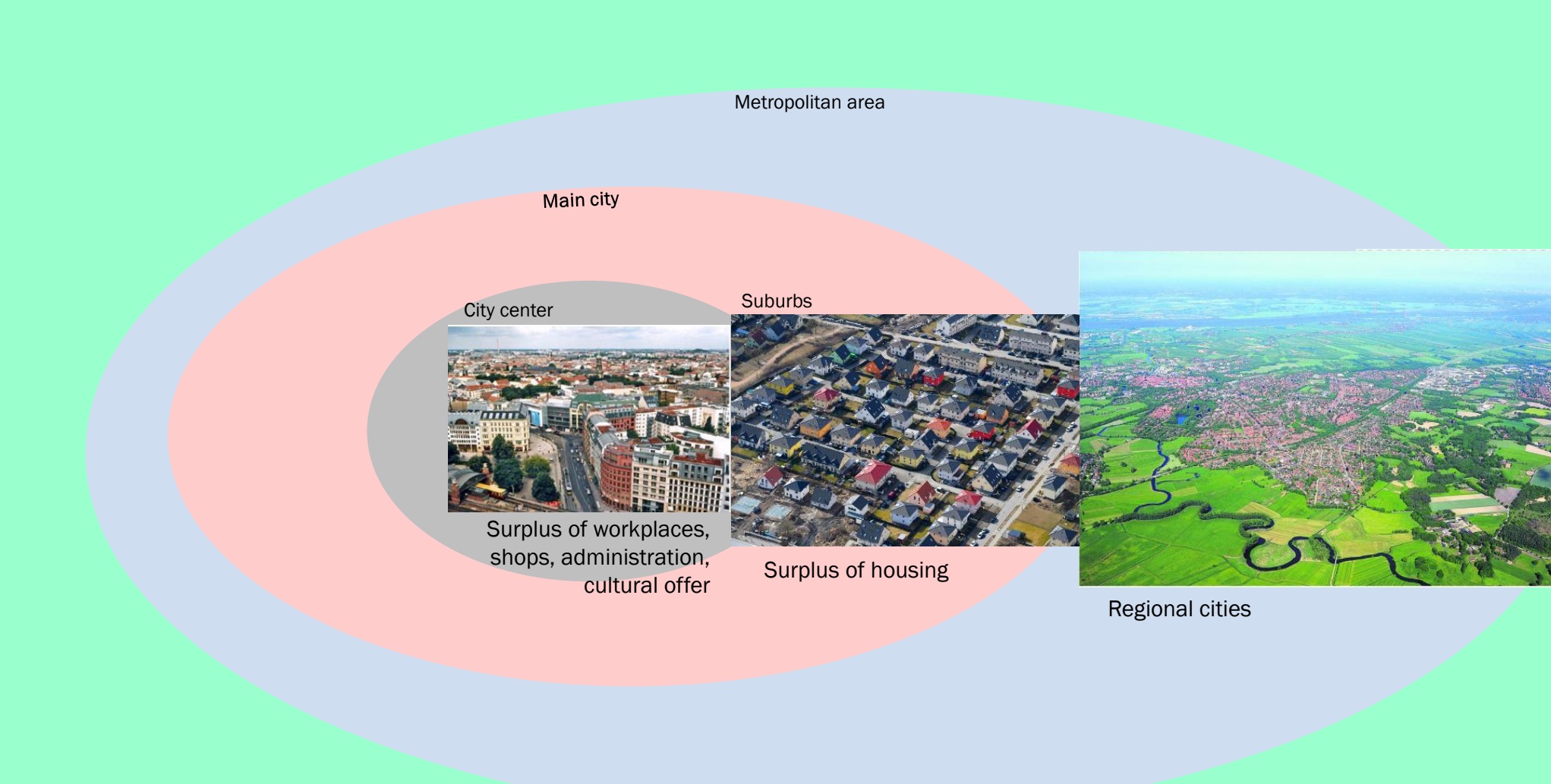
For passenger services, the market segmentation is not only geographical; it also reflects the stopping pattern, journey purpose, and frequency expectation of the service. Figure 6.2 maps the main passenger-service relations used in the planning discussion below. The area labels are storby-sentrum (metropolitan/city centre), forstad (suburb), and regionalt omland (regional hinterland or surrounding region).

Figure 6.2 Passenger railway market segments in Norway. Norwegian labels translated: fjerntog (long-distance trains), tilbringertog til lufthavn (airport feeder/airport-express trains), regionekspresstog i storbyregion (regional express trains in metropolitan regions), regiontog i/utenom storbyregion (regional trains inside/outside metropolitan regions), and lokaltog (local trains).

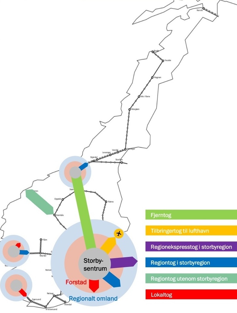
Passenger services are grouped by the scale of the trip and the role of the service in the network:

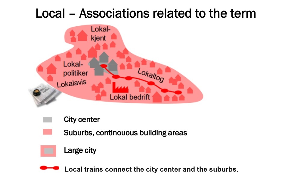
1. Local trains (lokaltog): Connect city centres with suburbs and continuously built-up areas. Characterised by high frequency, many stops, and short journey times. Examples: Oslo – suburbs, Bergen – Arna.

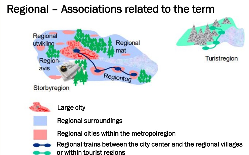
2. Regional trains (regiontog): Connect the city centre with surrounding regional cities and towns; also serve tourist routes. Passengers can leave their local area and return the same day. Examples: Oslo – Kongsberg, Trondheim – Steinkjer, Myrdal – Flåm.

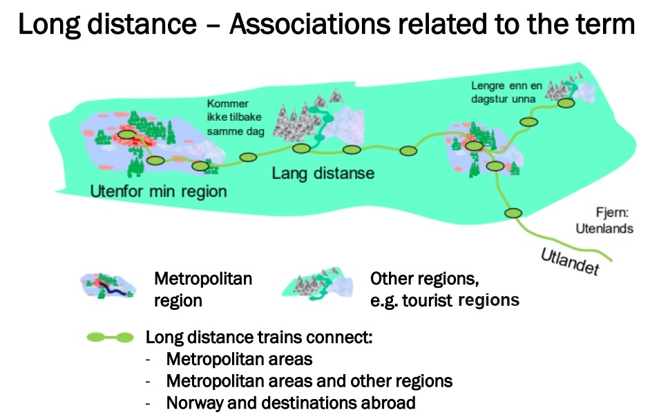
3. Long-distance trains (fjerntog): Connect metropolitan areas with other regions or abroad. Examples: Oslo – Bergen, Oslo – Trondheim, Trondheim – Bodø.

Figures 6.3–6.5 show the same classification as schematic service patterns: local trains concentrate on dense urban access, regional trains connect the city with its wider hinterland, and long-distance trains connect metropolitan areas and regions.

Figure 6.3 Local train services: short-distance, high-frequency connections between the city centre and suburbs or continuously built-up areas.

Figure 6.4 Regional train services: connections between a large city, regional surroundings, regional towns, and tourist regions.

Figure 6.5 Long-distance train services: connections between metropolitan areas, other regions, tourist regions, and destinations abroad.

The transport relation concept is used in Norwegian railway planning: each pair of origin and destination areas (with their "areas of influence") constitutes one transport relation. This is a planning concept rather than a capacity formula: it helps define which markets a train service is intended to serve. Some pairs of areas have no rail connection because the detour via other cities makes rail unattractive. This can be described as a transport-current analogy: differences in the distribution of workplaces, services, housing, and regional functions create transport flows between areas. Figure 6.6 visualises this idea by treating travel demand as a current created by differences between urban centres, suburbs, and regional surroundings.

Figure 6.6 Potential difference causes transport current: differences between city centres, suburbs, regional surroundings, and other regions create travel demand.

6.2.2.2 Freight Transport

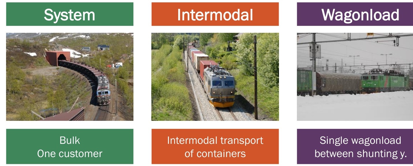
Freight capacity depends on the type of freight service, because system trains, intermodal trains, and wagonload trains have different terminal needs, train lengths, and timetable flexibility. Figure 6.7 separates these three freight categories.

Figure 6.7 Three categories of freight trains: system trains (bulk, single customer), intermodal trains (containers, swap bodies, trailers), and single wagonload trains.

Freight transport is categorised as:

• System trains (systemtog): Bulk transport for a single customer (ore, jet fuel, timber, cars, limestone, acid). Full trainloads between two fixed terminals (e.g., mine to factory or port). No shunting required.

• Intermodal trains (kombitog): Transport of containers, swap bodies, and trailers in fixed wagon trains between intermodal terminals over long distances. The most common freight category in Norway.

• Single wagonload trains (vognlasttog): Individual wagons carrying different goods travel between shunting yards, where wagons interchange between freight trains to reach their final destination. The smallest sending unit is one freight wagon.

For capacity analysis, the important point is not the total number of possible freight relations, but how each relation is operated: as a full system train, an intermodal path between terminals, or a wagonload movement requiring shunting and yard capacity.

6.3 Infrastructure and Signalling: The Minimum Headway

Before capacity can be calculated, the signalling constraint on train separation must be established. The minimum headway is the operational link between infrastructure layout and timetable capacity.

6.3.1 Blocking Sections and Signalling

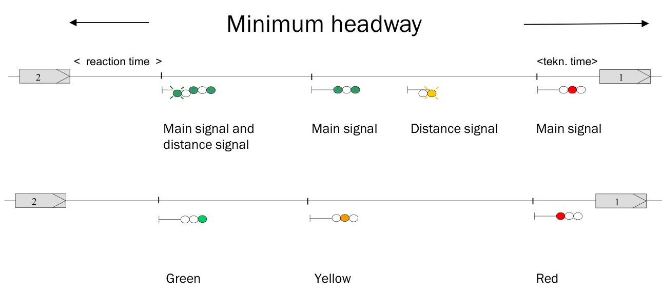
Railway lines are divided into blocking sections separated by signals [65]. A train occupies a blocking section and clears it before the next train may enter. The Norwegian signalling system (as of the current Automatic Train Control (ATC) era) uses a multi-aspect system:

Figure 6.8 relates the signal aspects to the protected distance that must be kept between successive trains in fixed-block operation. The upper row shows the physical signalling equipment along the track: main signals, distant signals, and a combined main/distant signal. The lower row removes the equipment names and keeps only the colour states used for the headway logic: green means the following train may proceed, yellow means the driver must be prepared to stop at the next main signal, and red means the block ahead is protected because the preceding train has not yet cleared it.

Figure 6.8 Signal aspects and the protected distance that determines minimum headway in fixed-block signalling. The upper row shows the physical signal sequence; the lower row shows the same situation simplified into green, yellow, and red signal states.

6.3.2 Calculating Minimum Headway

The minimum headway \(t_\mathrm{min}\) is the shortest possible time interval between two successive trains passing the same point. In a simplified fixed-block calculation it is determined by the protected distance that must be clear ahead of the following train:

Figure 6.9 translates this protected distance into the simplified headway-distance model used in Eq. 6.1.

Figure 6.9 Minimum-headway distance: reaction distance, two protected braking-distance blocks, train length, and technical time.

\[ d_\mathrm{headway} = d_\mathrm{reaction} + 2b + l_\mathrm{train} + v\,t_\mathrm{tech} \label{eq:headway_dist} \]

\[ t_\mathrm{min} = t_\mathrm{reaction} + \frac{2b + l_\mathrm{train}}{v} + t_\mathrm{tech} \label{eq:headway_time} \]

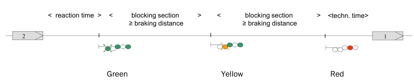
The terms in Eqs. 6.1–6.2 follow the left-to-right sequence in Figure 6.9. First, \(d_\mathrm{reaction}=v\,t_\mathrm{reaction}\) is the distance travelled during the driver's reaction time. Second, \(2b\) represents two protected braking-distance blocks in the simplified two-block model. Third, \(l_\mathrm{train}\) is the length of the preceding train that must clear the protected section. Finally, \(v\,t_\mathrm{tech}\) is the distance equivalent of the technical safety margin \(t_\mathrm{tech}\), where \(v\) is the train speed. Dividing the distance terms by \(v\) gives Eq. 6.2: reaction time, protected blocking-section time, and technical time.

In an actual blocking-time calculation the protected distance and time also include route setting, signal sighting or cab-signalling supervision, overlap or safety distance, detection-section release, train-length clearance, braking-curve margins, and station dwell time if the headway is measured through a stop. If the signal spacing is not equal to the braking distance, the term \(2b\) must be replaced by the actual protected block or detection-section sequence. On modern Norwegian main lines with ATC, minimum headways are typically of the order of 4–6 minutes on single-track lines and 2–3 minutes on double-track lines [141, 29].

6.4 System Approach to Capacity

Capacity should be treated as a system property rather than as a property of a single track section. The limiting element may be a line, station, terminal, depot, or operational dependency.

6.4.1 The Capacity Chain

Railway traffic capacity is not determined by a single element but by the entire chain of system components. The total traffic capacity equals the capacity of the weakest link in the chain:

The principal capacity-determining components are:

• Line capacity: The number of trains that can pass along a section of line per unit time, determined by minimum headway, speed differences between train types, and the number of tracks

• Station capacity: Platform tracks, crossing loops, turnout geometry, and dwell time determine how many trains can be accommodated simultaneously

• Turnaround capacity: At terminal stations, trains must be turned or shunted for the return journey; this limits the frequency of services

• Train yard (depot) capacity: Stabling and servicing capacity for trainsets during off-peak hours

• Maintenance facility capacity: Workshop access for heavy maintenance

• Communication capacity: Data links for signalling and train management

• Traction energy capacity: Power supply from the catenary system

6.4.2 Dependencies and Junctions

A key concept in railway capacity planning is dependency: when two train paths share a section of track (a junction, a single-track section, or a station), changes to one train path affect all others that use the shared resource.

6.4.2.1 Junctions

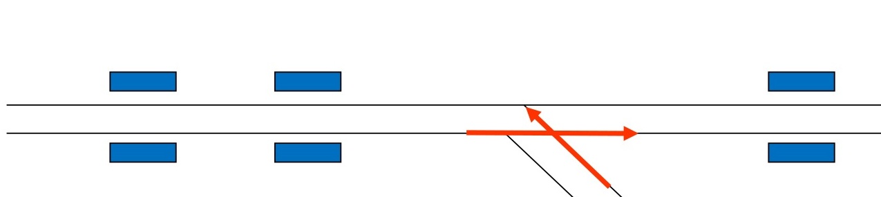
A flat junction keeps the conflicting route movements at the same level, so crossing and merging trains remain mutually dependent. Figure 6.10 shows this capacity constraint schematically.

Figure 6.10 Level junction (flat junction): crossing and merging moves remain mutually dependent because routes conflict at the same level.

A flying junction removes the same conflict by separating the route movements vertically; Figure 6.11 shows why this gives more independent train paths and therefore more timetable freedom.

Figure 6.11 Flying junction (grade-separated junction): routes are separated vertically, reducing timetable dependencies and permitting shorter headways.

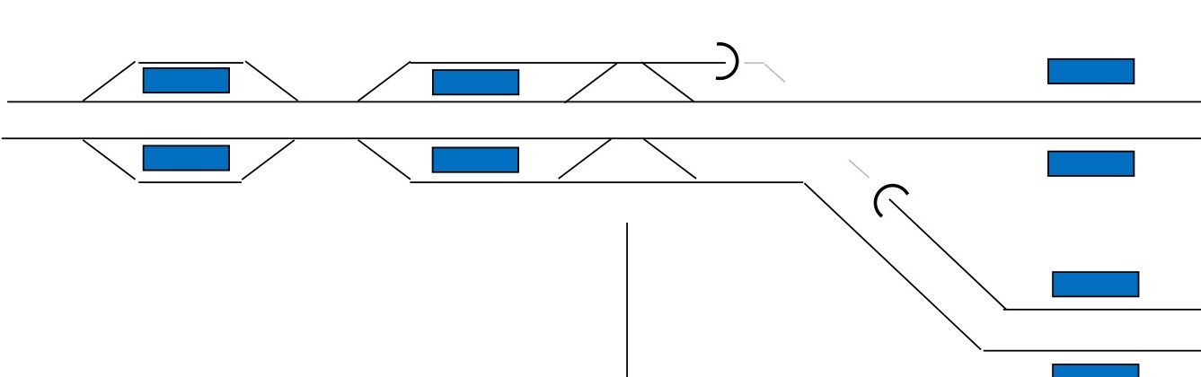
The Ski station (south of Oslo) provides a contemporary Norwegian example: the new Follo line separates fast regional traffic from local Østfold traffic and reduces the number of conflicting moves in the station throat. The achievable headway is therefore in the few-minute range, but the exact value depends on the timetable pattern, stopping pattern, platform occupation, station throat layout, signalling, and turnback requirements. A level junction would preserve more route conflicts and therefore consume more capacity.

6.4.2.2 Remerging Lines

When two separate lines merge into a shared section, all timetables on both lines become mutually dependent through the shared section. If one line is delayed, it may block the shared section and cascade delays to the other. For robust timetabling, railway lines should be separated on the entire network where possible, a principle underlying major Norwegian infrastructure investments such as the Follo line.

6.5 Theoretical and Practical Capacity

Capacity figures are useful only when their assumptions are clear. This section distinguishes idealised theoretical capacity from the practical capacity that remains after robustness and timetable constraints are considered.

6.5.1 Theoretical Capacity (UIC 405E)

The theoretical capacity [65, 161] \(K\) of a line section is the maximum number of trains that can be operated during an analysis period \(T\), given a minimum headway \(t_m\):

\[ K = \frac{T}{t_m} \label{eq:theoretical_capacity} \]

Figure 6.12 shows the idealised case behind Eq. 6.3: the analysis period is filled by train paths spaced only by the minimum headway.

Figure 6.12 Theoretical capacity: the analysis period T is divided by the minimum headway t_m to give the maximum number of trains.

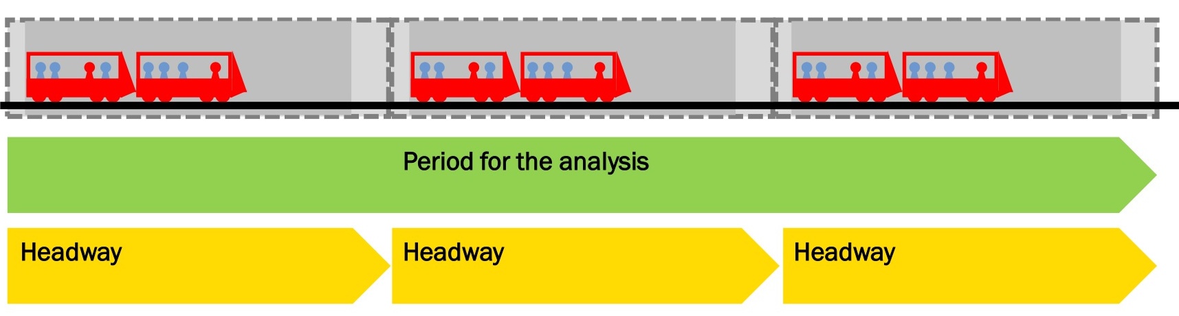
The theoretical capacity represents the absolute maximum, it leaves no time for delays to recover. Operating at theoretical capacity means that a single delay to any train propagates directly to all following trains.

6.5.2 Practical Capacity and Buffer Time

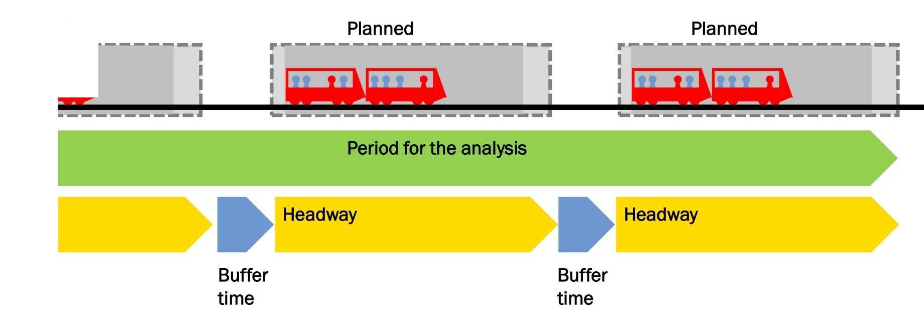
The practical capacity \(K_p\) is the number of trains that can realistically be operated with acceptable punctuality [161, 141]. It is obtained by introducing a buffer time \(t_\mathrm{buff}\) between successive trains:

\[ K_p = \frac{T}{t_m + t_\mathrm{buff}} \label{eq:practical_capacity} \]

Figure 6.13 shows how the same train paths consume more time once buffer margins are inserted to absorb small disturbances.

Figure 6.13 Practical capacity: buffer times are inserted between train paths, allowing small delays to be absorbed without propagating to following trains.

6.5.3 Mixed Traffic: Speed Differences

On lines with both fast and slow trains (mixed traffic), the minimum headway is not the same for all train pairs. When a fast train follows a slow train on the same track on double track, or when a freight train blocks a crossing loop on single track, the effective headway is larger than the pure minimum headway.

For double-track, mixed traffic, a preliminary capacity approximation is:

Figure 6.14 explains the reason for the extra term in the approximation: different train-path slopes create unused spacing when fast and slow trains share the same track pair.

Figure 6.14 Double-track capacity is reduced when mixed traffic creates unequal train-path slopes and larger effective headways.

\[ K_{\mathrm{double,approx}} = \frac{T}{t_m + 0.5\,\Delta t} \label{eq:double_track} \]

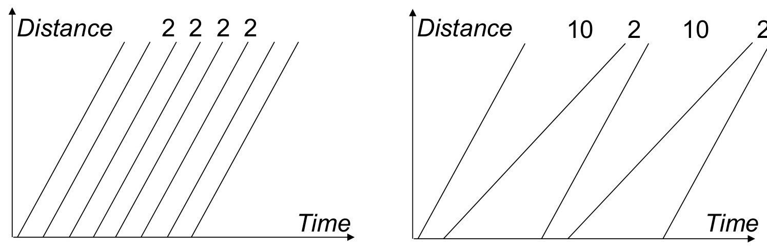
where \(\Delta t\) is the difference in running time between the fast and slow train over the section. This approximation assumes a regular alternation of fast and slow trains in one direction, no overtaking within the analysed section, and no additional constraints from platform occupation, junctions, turnbacks, or dwell-time variation. It is therefore useful for first estimates, but it is not a substitute for blocking-time analysis, UIC 406 compression, or microscopic timetable simulation. When buffer time is also required (to ensure punctuality), the practical capacity for mixed-traffic double track combines both penalties:

\[ K_{p,\mathrm{double,approx}} = \frac{T}{t_m + 0.5\,\Delta t + t_\mathrm{buff}} \label{eq:double_track_practical} \]

Equations 6.5–6.6 should be read as a mixed-traffic penalty model. The denominator contains three effects: the minimum separation \(t_m\), the extra spacing caused by the running-time difference \(0.5\,\Delta t\), and the punctuality reserve \(t_\mathrm{buff}\). If fast and slow trains continue to share the same double-track pair, all three terms consume capacity.

A useful comparison is a separated-operation benchmark. Suppose the fast trains and slow trains no longer share the same track pair. This could be achieved by a four-track corridor, where one double-track pair is used by fast trains and the other by slow trains. The important capacity principle is not the number four itself, but the removal of the mixed-traffic term: once the two service groups are separated, \(\Delta t\) no longer reduces capacity on a shared track. The two service groups can then be estimated separately and added:

\[ K_{p,\mathrm{separated}} = \frac{T}{t_m^\mathrm{fast}+t_\mathrm{buff}} + \frac{T}{t_m^\mathrm{slow}+t_\mathrm{buff}} \]

This is an idealised comparison, not a design capacity. In a real corridor, station throats, platform occupation, junctions, turnbacks, depot movements, and uneven stopping patterns may still become the controlling capacity constraints.

6.5.4 Single-Track Capacity: Crossing Patterns

For single-track lines, capacity is governed by the crossing pattern and by the longest critical section between crossing opportunities:

Figure 6.15 shows why the controlling quantity on single track is not a simple following headway, but the repeat time needed for trains to meet at feasible crossing locations. The figure should be read as a simplified graphic timetable: the vertical axis is location, the horizontal axis is time, and each diagonal line is one train movement between stations. Opposing train paths cannot cross in the open line, so a train in the opposite direction can only be released after the previous train has reached a station or crossing loop and the route has been cleared.

Figure 6.15 Single-track capacity is governed by feasible crossing patterns between stations and by the longest critical running-time cycle.

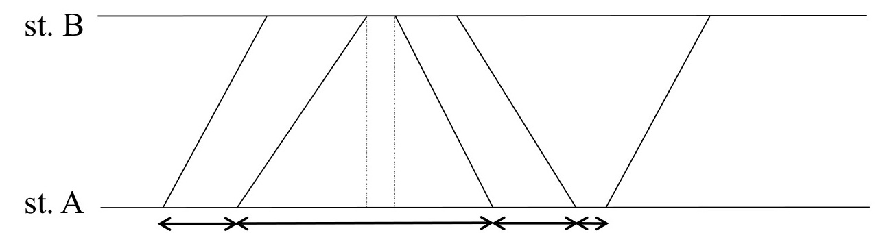
The horizontal arrows at the bottom indicate the time intervals that must be respected before the next train movement can start. In double-track operation, capacity is often estimated from the minimum following headway between trains in the same direction. On single-track lines, the more important quantity is the cycle time: the time needed to complete a feasible sequence of movements and crossings. The longest such cycle on the line becomes the bottleneck, because every other train has to fit around it.

\[ K_\mathrm{single} \approx \frac{T}{t_\mathrm{cycle}+t_\mathrm{buff}} \label{eq:single_track} \]

where \(t_\mathrm{cycle}\) is the minimum repeat time for one feasible meeting pattern, including running time to the crossing station, route setting/release, train length clearance, dwell or crossing time, and any reversal of direction in the timetable graph. The line is divided into sections of similar traffic conditions; the section with the largest compressed cycle time governs. A single average headway is therefore usually insufficient for single-track design.

6.5.5 Utilisation and Robustness as Screening Concepts

After a practical capacity has been estimated, the next question is how heavily that capacity is used. A simple utilisation factor compares the planned number of trains with the estimated practical capacity:

\[ u = \frac{N_\mathrm{planned}}{K_p} \]

where \(N_\mathrm{planned}\) is the planned number of train paths per hour (or per analysis period) and \(K_p\) is the practical capacity estimate for the same period. A value close to 1 means that most of the available capacity is used.

Robustness means the ability of the timetable to absorb small delays without spreading them to other trains. A low utilisation leaves recovery margin; a high utilisation leaves little space for late trains, longer dwell times, or small operational disturbances. As a first screening rule, mixed-traffic peak-hour timetables should normally stay below about 70–75 % utilisation before they are accepted for detailed timetable design. More formal checks are introduced later through UIC 406 compression (Section 6.6) and delay propagation (Section 6.7).

Worked Example: Mixed-Traffic Capacity Screening

Question. A corridor carries regional express and local stopping trains on the same double-track pair. Over the analysed section, use:

\[ \begin{aligned} t_\mathrm{express} &= 18\,\mathrm{min}, & t_\mathrm{local} &= 26\,\mathrm{min},\\ t_m &= 2.5\,\mathrm{min}, & t_\mathrm{buff} &= 0.5\,\mathrm{min},\\ T &= 60\,\mathrm{min}. \end{aligned} \]

(a) Estimate the practical capacity when the express and local trains are mixed.

(b) As a comparison, estimate the practical capacity if the two service groups are fully separated so that express trains and local trains no longer share the same track pair. Use \(t_m^\mathrm{express}=2.5\) min and \(t_m^\mathrm{local}=3.0\) min.

(c) A proposed peak timetable contains 7 trains/hour per direction on the mixed double-track line. Comment on the utilisation and robustness.

Solution.

(a) Practical capacity with mixed traffic. The running-time difference between the local and express train is:

\[ \Delta t = 26 - 18 = 8\ \mathrm{min} \]

Using Eq. 6.6, the mixed-traffic practical capacity is:

\[ K_p^\mathrm{mixed} = \frac{60}{2.5 + 0.5\cdot 8 + 0.5} = \frac{60}{7.0} = 8.6\ \text{trains/h per direction} \]

Answer to (a): the simplified practical capacity is 8.6 trains/h per direction. As a timetable screening value, this should be interpreted as approximately 8 train paths per hour per direction after rounding to whole train paths and allowing for detailed timetable constraints.

(b) Practical capacity with separated operation. This part is not another mixed-traffic calculation. It asks what happens if the express and local trains are operated on independent track pairs. Then the running-time difference \(\Delta t\) is no longer a penalty in the denominator, because the two service groups do not have to follow one another on the same track:

\[ K_p^\mathrm{express} = \frac{60}{2.5 + 0.5} = 20.0\ \text{trains/h} \]

\[ K_p^\mathrm{local} = \frac{60}{3.0 + 0.5} = 17.1\ \text{trains/h} \]

\[ K_p^\mathrm{separated} = 20.0 + 17.1 = 37.1\ \text{trains/h per direction} \]

Answer to (b): the separated-operation benchmark gives 37.1 trains/h per direction. If this separation were implemented physically as a four-track corridor, this value would represent the idealised four-track comparison. The purpose of the calculation is to show the capacity effect of removing the mixed-traffic penalty, not to claim that every double-track line should be upgraded to four tracks.

(c) Utilisation and robustness of the proposed mixed timetable. The utilisation of the proposed 7 trains/h service is calculated against the mixed-traffic capacity from part (a):

\[ u = \frac{7}{8.6} = 0.81 \]

Answer to (c): the proposed timetable uses about 81 % of the simplified practical capacity estimate. This exceeds the usual 70–75 % peak-hour robustness target for mixed traffic. The timetable may be possible on paper, but it has little recovery margin.

Before accepting it, the planner should run a detailed UIC 406 compression study and conflict analysis. The worked example demonstrates the key operational consequence: speed differences do not only increase journey time for the slower train, they also consume capacity for the faster train following behind.

Worked Example: Stop Pattern and Mixed-Traffic Capacity

Question. A double-track line has one track per direction. In each repeating service interval \(T_\mathrm{int}\), one local train and one regional train depart in the same direction. The local train stops at \(n\) intermediate halts, and each additional stop adds 2.0 min to its running time. The minimum headway is 1.5 min and a 0.5 min buffer is provided after each of the two trains. Determine how the maximum integer value of \(n\) depends on \(T_\mathrm{int}=10\), 15, and 20 min for three stopping patterns.

For a two-train repeating pattern, it is clearer to write the period directly as

\[ T_\mathrm{int}=t_{L\rightarrow R}+t_{R\rightarrow L}+2t_\mathrm{buff}, \label{eq:stop_pattern_interval} \]

where \(t_{L\rightarrow R}\) is the separation required when the local train runs first and \(t_{R\rightarrow L}\) is the separation when the regional train runs first. This is the same occupation logic as the UIC 405E screening method, written so that the two train sequences and both buffers remain visible.

Case A: the regional train runs non-stop. When the local train runs first, the regional train must recover the local train's \(2n\)-minute stopping-time penalty before the minimum headway is restored:

\[ t_{L\rightarrow R}=2n+1.5,\qquad t_{R\rightarrow L}=1.5. \]

Therefore,

\[ T_\mathrm{int}=(2n+1.5)+1.5+2(0.5)=2n+4, \qquad n_\mathrm{max}=\left\lfloor\frac{T_\mathrm{int}-4}{2}\right\rfloor. \]

Case B: the regional train shares one intermediate stop. The running-time difference is now \(2(n-1)\) rather than \(2n\):

\[ t_{L\rightarrow R}=2(n-1)+1.5,\qquad t_{R\rightarrow L}=1.5, \]

which gives

\[ T_\mathrm{int}=2n+2, \qquad n_\mathrm{max}=\left\lfloor\frac{T_\mathrm{int}-2}{2}\right\rfloor. \]

Case C: the shared stop becomes a directional bottleneck. In the opposite direction, the regional train stops at the first halt after the origin and occupies the only available platform face. The regional-first sequence therefore needs the 1.5 min minimum headway plus 2.0 min dwell/clearance time:

\[ t_{L\rightarrow R}=2(n-1)+1.5,\qquad t_{R\rightarrow L}=1.5+2.0=3.5. \]

The period becomes

\[ T_\mathrm{int}=2n+4, \qquad n_\mathrm{max}=\left\lfloor\frac{T_\mathrm{int}-4}{2}\right\rfloor. \]

Stopping pattern	Tint [min]
2-4	10	15	20
A: regional train non-stop	3	5	8
B: one shared regional stop	4	6	9
C: shared stop constrains the reverse direction	3	5	8

Table 6.1 Maximum number of intermediate local-train stops in the three worked cases.

Interpretation. Harmonising the stopping patterns in Case B permits one additional local stop at each service interval without changing the infrastructure. Case C shows why that gain is not guaranteed in both directions: platform occupation at one halt can consume the recovered margin. The calculation must therefore be checked in both directions on a graphic timetable. For a complete line section, the same logic must include crossing patterns and route-specific constraints.

6.6 Capacity Analysis Methods

The methods below translate timetable structure into capacity consumption. They are mainly used to compare alternatives and identify where recovery margins become too small.

6.6.1 UIC 406: The Compression Method

The UIC 406 method evaluates capacity consumption by compressing the graphic timetable:

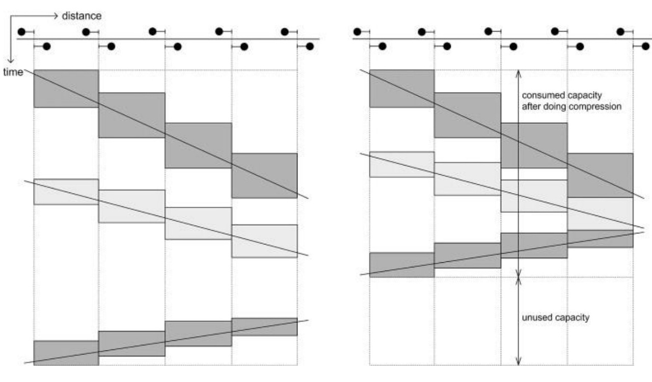
The compression principle is shown in Figure 6.16: timetable gaps that are not required by signalling or operating constraints are removed, leaving the infrastructure occupation time. The diagonal lines are train paths in a distance-time diagram, while the grey blocks represent the time during which each train occupies the relevant infrastructure according to the signalling and route-setting constraints. In the right-hand part, the train paths have been shifted closer together without changing their order and without violating the required minimum headways or blocking times.

The key idea of UIC 406 is that compression removes unused gaps, but it does not invent a new timetable or change train running times. The vertical arrow labelled "consumed capacity" is the compressed infrastructure occupation time, \(t_\mathrm{compressed}\). The remaining space in the analysis period is the unused capacity, which can provide recovery margin or allow additional train paths if other constraints also permit it.

Figure 6.16 The UIC 406 compression method: all train paths on a line section are moved together (compressed) as tightly as the minimum headways allow.

The capacity consumption index [161] is:

\[ U = \frac{t_\mathrm{compressed}}{T_\mathrm{analysis}} \label{eq:capacity_consumption} \]

UIC 406 gives recommended capacity-consumption values rather than universal pass/fail limits. The commonly used interpretation distinguishes peak-hour and daily analysis windows, with stricter utilisation limits for mixed-traffic lines.

Line type	Peak hour	Daily period
Dedicated suburban passenger traffic	85 %	70 %
Dedicated high-speed traffic	75 %	60 %
Mixed-traffic lines	75 %	60 %

Table 6.2 Typical UIC 406 guideline values for maximum infrastructure occupation. The values are screening benchmarks; national rules, punctuality targets, traffic mix, and timetable robustness may require lower values.

Values above the relevant guideline do not automatically mean that a timetable is impossible, but they indicate little recovery margin and require timetable-specific delay and robustness analysis.

The compression method is particularly useful for evaluating existing or planned timetables on complex networks.

6.6.2 Graphic Timetable

The graphic timetable (also called the train graph or string diagram) is a distance-time diagram showing the path of each train through a line section:

Figure 6.17 shows how this distance-time representation makes different speeds, stopping patterns, and potential conflicts visible in one diagram.

Figure 6.17 Graphic timetable for a double-track line section with local trains stopping at intermediate halts and regional trains running express.

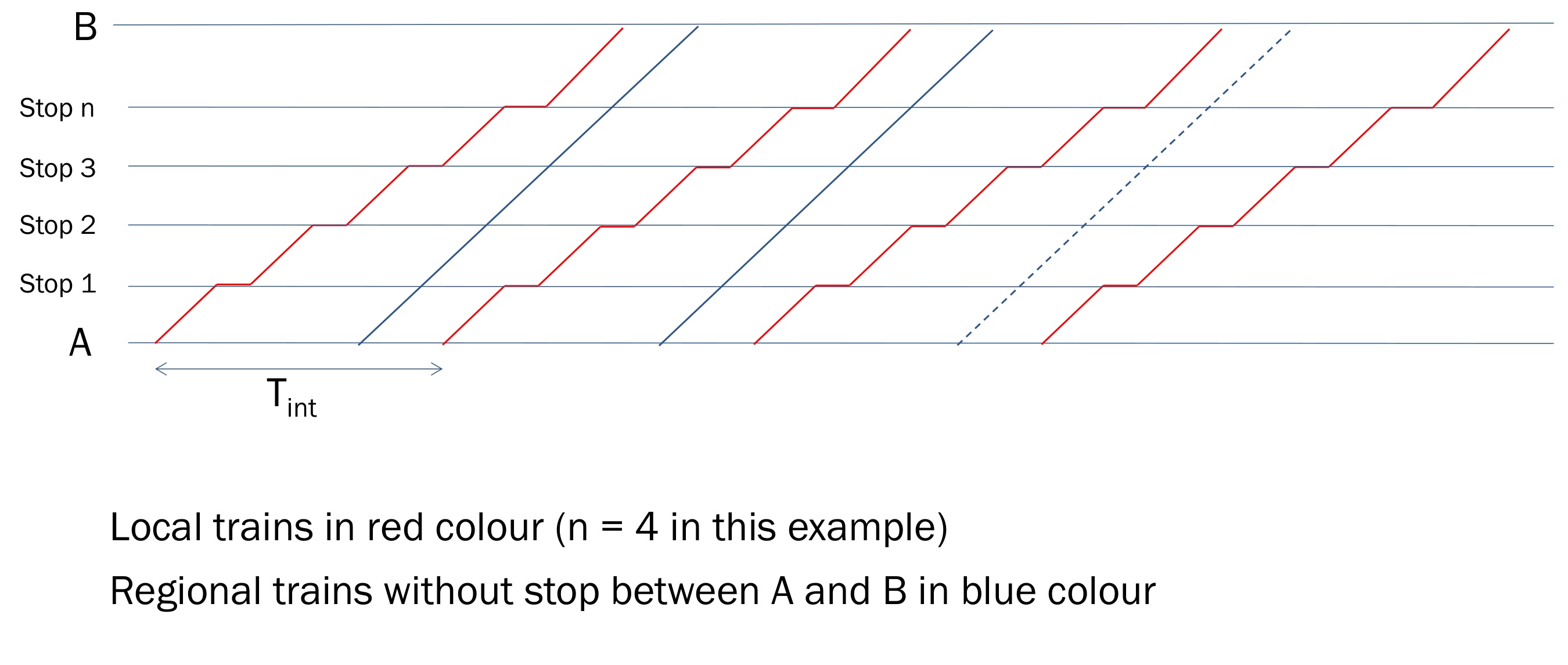
In the graphic timetable, each train appears as a diagonal line whose slope represents its speed. Steeper lines indicate higher speed. Two lines that cross represent a potential conflict (two trains at the same location at the same time) [65]; on single-track lines, all train pairs must cross at designated crossing loops. The graphic timetable makes capacity conflicts immediately visible.

6.7 Punctuality and Delay Propagation

High capacity utilisation reduces the room available for recovery. The following concepts explain how small disturbances can spread through a railway network.

6.7.1 Delays and Propagation

A railway system operating at or near capacity is sensitive to delays. When one train is delayed, it may occupy a blocking section longer than planned, forcing the following train to slow down or stop. This delay propagation (forsinkelsessmitte) [141] can spread through the network.

Figure 6.18 shows the nonlinear relationship between capacity utilisation and delay propagation: as the line approaches full occupation, each primary delay creates progressively more secondary delay.

Figure 6.18 Delay propagation factor as a function of utilisation factor for harmonised double-track operation.

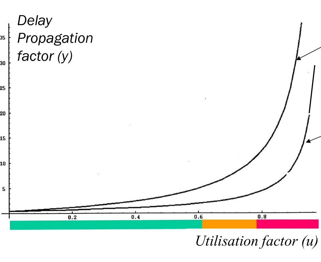
The delay propagation factor \(\gamma\) is:

\[ \gamma = \frac{\sum \text{all delays}}{\text{initial delay}} \label{eq:propagation_factor} \]

As the utilisation factor \(u = K/K_\mathrm{max}\) approaches 1, the propagation factor increases rapidly. A larger initial delay relative to the minimum headway produces stronger secondary-delay propagation for the same utilisation level. This is the fundamental reason why railway lines should never be operated at their theoretical capacity: the system becomes extremely fragile, and small disruptions cause large-scale delays.

Practical guidelines for Norwegian main lines target a utilisation factor of no more than 0.70–0.75 (70–75 % of theoretical capacity) during the peak hour to maintain acceptable punctuality [161, 124].

6.7.2 Lateness and Delay Definitions

Norwegian railway statistics distinguish between [29, 26, 21]:

• Punctuality: The proportion of trains that arrive at their final destination, and at Oslo S where relevant, within 3:59 minutes for most passenger trains and within 5:59 minutes for long-distance, freight, and cross-border trains. The national punctuality target for passenger traffic is typically around 90 %.

• Primary delay: A delay caused by an event (technical failure, signal fault, operational error, external cause) that directly affects one train.

• Secondary (propagated) delay: A delay caused to a train by another train's primary or secondary delay.

• Regularity: The proportion of trains actually operated (not cancelled).

6.8 Impact of ETCS/ERTMS on Capacity

The European Train Control System (ETCS, operating under the ERTMS umbrella standard) is being progressively deployed on the Norwegian network; the signalling architecture is described in Chapter 11, while this section focuses on the capacity effect. ETCS Level 2 replaces lineside signal aspects with movement authorities shown in the driver's cab and transmitted by radio between the radio block centre (RBC) and the train's on-board computer. Train position is estimated on board and corrected by balises, while Level 2 operation normally still relies on trackside train detection such as axle counters or track circuits.

Key capacity effects of ETCS compared to the existing ATC system:

Negative effects:

• Braking curves in ETCS are more conservative (mathematically precise), leading to more restrictive speed profiles than ATC in some situations

• Continuous speed supervision means that the train must slow down earlier when approaching a stop signal

Positive effects:

• Simultaneous entry at crossing loops becomes possible without constructing longer loop tracks where the interlocking, release speed, marker-board location, route overlap, and safety distance are designed for it

• In some cases, higher permitted speeds for freight trains (whose braking capability may be underestimated by ATC's distance-signal-based system)

• Reduced dependence on fixed trackside equipment reduces the risk of signal failures

The net capacity effect of ETCS depends strongly on line characteristics, train mix, block-section design, braking curves, release speeds, and RBC/interlocking parameter settings. On heavily loaded Norwegian lines, ETCS should therefore be treated as a layout-specific capacity measure rather than as a general capacity increase.

6.9 Planning Horizon

Capacity analysis is carried out for multiple planning horizons:

• Short-term (current year and 1–3 years): Timetable planning and slot allocation. Uses UIC 406 compression analysis on the existing timetable.

• Medium-term (5–10 years): Infrastructure development planning. Uses simplified analytical formulas, blocking-time analysis, and UIC 406 compression to assess whether planned traffic volumes can be accommodated.

• Long-term (10–30 years): Strategic planning for major infrastructure investments. Uses traffic demand forecasts (low/average/high scenarios) to size new lines and stations.

Long-term planning must address the entire range of possible market developments. Three scenarios (low, average, high) are typically evaluated to bound the uncertainty in future traffic volumes.

6.10 Chapter Summary

Capacity concept. The same track layout can carry different numbers of trains depending on stopping patterns, speed differences, signalling, junction conflicts, platform occupation and recovery margins. The chapter therefore connects railway infrastructure to operation: a line with good physical geometry may still have limited capacity if the timetable creates repeated conflicts or if trains with very different speeds share the same path.

Headway. Minimum headway depends on block length, braking distance, signal spacing, train length, speed, dwell time and route release. Reducing headway can increase theoretical capacity, but only if the operating pattern remains stable. In stations and junctions, the controlling headway may be set by route conflicts or platform occupation rather than by plain-line block sections.

Mixed traffic. Fast passenger trains, stopping local trains and slower freight trains interact because they occupy track sections for different durations and catch up with one another at different rates. Overtaking opportunities, crossing loops, passing patterns and service priorities therefore become central design and timetable issues. A small speed difference may be manageable, while a large speed difference can dominate the capacity of an otherwise well-equipped line.

Practical capacity. A timetable that fills every possible train path has no resilience against delays. Buffer time, recovery margins and regularity requirements reduce usable capacity, but they are necessary for reliable operation. UIC capacity methods, compression analysis and graphic timetables help show how much of the theoretical capacity is already consumed and where additional trains would make the service fragile.

Robustness. The goal is not simply to maximise the number of train paths, but to provide a timetable that can recover from small disturbances while serving passenger and freight needs. Single-track crossing patterns, junction design, platform use, remerging lines and delay propagation all influence this balance. Capacity planning is therefore an operational design process as much as a calculation exercise.

Assignments

Assignment 1: Mixed-speed double-track capacity

A double-track line carries fast trains (running time A–B: 20 min) and slow trains (running time A–B: 30 min) in each direction. The minimum headway is 2 min and the buffer time is 0.5 min.

(a) Calculate the practical capacity using the simplified mixed-traffic formula.

(b) As a comparison, suppose fast and slow trains are fully separated onto independent track pairs (for example in a 4-track corridor). With headways of 2 min for fast trains and 3 min for slow trains, what is the new practical capacity?

(c) What is the percentage increase in capacity?

Assignment 2: Single-track crossing capacity

A single-track line section between stations A and B has a running time of 12 min (A to B) and 14 min (B to A). Crossing time at each station is 2 min. Buffer time is 1 min and the analysis period is 60 min.

(a) Calculate the weighted average minimum headway \(t_m\).

(b) Determine the theoretical and practical capacity (trains per hour in total, both directions).

(c) What additional crossing loop halfway between A and B would do for capacity? (Qualitative reasoning only.)

Assignment 3: UIC 406 capacity utilisation

A timetable study using UIC 406 on a busy suburban line gives a compressed occupation time of 52 minutes in the peak hour.

(a) Calculate the capacity consumption index \(U\).

(b) According to UIC 406 guideline values, is this acceptable?

(c) The operator wants to add 2 more trains per hour to the peak service. Each additional train adds approximately 2.5 minutes to the compressed time. Would this remain acceptable?

Assignment 4: Primary and secondary delay propagation

A freight train suffers a 10-minute primary delay on a busy single-track section. Use the delay-propagation concept in Figure 6.18 to explain what happens next.

(a) Define primary delay and secondary delay. Give one practical example of each.

(b) Using the delay propagation factor concept, explain why a 10-minute primary delay on a line with utilisation \(U = 0.80\) produces secondary delays significantly larger than on a line with \(U = 0.50\).

(c) What operational measures can reduce the propagation of secondary delays?

Assignment 5: Single-track capacity utilisation

A single-track line has a maximum line capacity of 48 trains per day. Currently 26 trains operate daily. A new freight contract will add 8 more trains per day.

(a) Calculate the utilisation factor before and after adding the freight trains.

(b) Using UIC 406 guideline values as a screening check, assess whether the line can absorb the additional traffic without exceeding acceptable daily capacity consumption.

(c) Describe two infrastructure measures that would increase the effective capacity of this line, and explain the mechanism behind each.

(d) Why is the relationship between utilisation and delay non-linear?