01

Railway Traffic Loading

Brief video explanation Watch video

1.1 Introduction

A railway is a guided transport system in which vehicles travel along a pair of fixed steel rails. Unlike road transport, the interface between the steel wheel and the steel rail is constrained both geometrically and mechanically: the rail head profile guides the wheel laterally, while the rail itself must carry and distribute all vertical, longitudinal, and lateral forces imposed by passing trains [68]. This interface has a contact patch typically smaller than a human thumbnail, yet it carries one wheel load at a time. For a 30 t axle load, each wheel contact transmits approximately 147 kN, making railway loading one of the most concentrated and frequently repeated load conditions in civil engineering.

Railway traffic loading encompasses all forces and load effects imposed on the track infrastructure as a result of the presence or movement of railway vehicles. A thorough understanding of these loads is required at every stage of railway engineering:

• Track design: Load calculations govern the selection of rail profile, sleeper type and spacing, fastening system, and required ballast depth.

• Bridge and structure design: Standardised load models (e.g. Load Model LM71 per EN 1991-2) are derived from traffic loading statistics.

• Maintenance planning: The rate of track geometry deterioration is directly related to traffic loading; heavier and faster trains degrade track faster.

• Safety assessment: Excessive stresses in rail or ballast can lead to rail fracture, track buckling, or subgrade failure, all of which are potential causes of derailment.

Traffic loads on a railway track are categorised into three groups according to their physical origin [130]:

1. Static loads: Gravitational forces from the dead weight of a stationary vehicle, determined entirely by the axle load distribution.

2. Quasi-static loads: Slowly varying forces that arise when a train negotiates a horizontal curve (centrifugal force) or is exposed to cross-winds. These forces cause a redistribution of load between inner and outer rails and between bogies.

3. Dynamic loads: Rapidly varying forces caused by track irregularities (corrugation, rail joints, switches), vehicle imperfections (wheel flats, out-of-round wheels), and speed-dependent resonance effects in the vehicle–track system. Dynamic loads are characterised by their statistical variability and are typically accounted for by means of a Dynamic Amplification Factor (DAF).

This chapter introduces the UIC wheel arrangement classification system, the mechanics of load distribution through the track structure, and the Eisenmann analytical method for calculating static and dynamic stresses in rail, sleepers, and ballast. Reference is made throughout to the requirements of Bane NOR technical regulations [10] and the Bane NOR Network Statement [30].

1.2 Railway Systems and Loading Characteristics

The term "railway" covers a wide range of guided transport systems with very different vehicle masses, axle loads, and operating speeds. The loading characteristics of a railway are determined by its operational purpose, and it is essential to understand these before undertaking any structural analysis. Three main categories are recognised [130]:

1.2.1 Urban and Commuter Railways

Urban and commuter railways include metro (underground/subway) systems, light rail transit (LRT), and tramways. These systems serve high-density urban passenger demand, operating at frequent headways over relatively short distances. Their principal characteristics are:

• Axle loads typically in the range 8–15 t

• Maximum speeds generally 80–120 km/h

• Dedicated infrastructure (segregated from road traffic in most cases)

• High service frequency, requiring robust and low-maintenance track

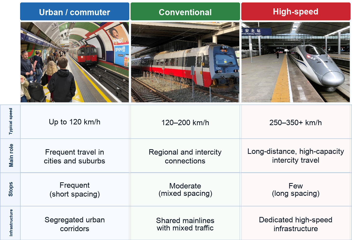
The comparison in Figure 1.1 should be read qualitatively rather than as a strict design chart. Urban and commuter railways are characterised by frequent stopping patterns and relatively low to moderate axle loads, while conventional and high-speed systems are shown as contrasts with higher operating speeds, longer station spacing, and stronger requirements for segregated infrastructure. The key engineering message is that the governing design problem changes with the service concept: urban systems are constrained by station spacing, tunnels, structures, and embedded or compact track forms, whereas conventional and high-speed lines must satisfy main-line structural, dynamic, and geometric requirements.

Figure 1.1 Passenger railway system categories and typical operating characteristics.

1.2.2 Conventional Railways

Conventional railways carry both intercity passenger trains and freight trains, typically on shared infrastructure. They form the backbone of the national railway network. Their loading characteristics span a wide range:

• Passenger train axle loads: typically 12–22.5 t; freight wagon axle loads: commonly 20–22.5 t on standard European main lines

• Maximum speeds: up to 210 km/h for passenger trains in Norway; typically 80–120 km/h for freight, with route-specific limits (Bane NOR Network Statement 2026 [30]; EU Infrastructure TSI performance categories [71])

• Mixed traffic requires track designed for both high speed and high axle load

The resulting trade-off between axle load and operating speed is summarised schematically in Figure 1.2.

Figure 1.2 Schematic axle-load and speed ranges for conventional railway operations. Standard European freight is shown around 20–22.5 t per axle, while high-speed passenger traffic uses comparatively low axle loads at much higher speeds [71, 70, 169].

1.2.3 Specialised Railways

Some railway systems are designed for a single dedicated purpose, and their loading characteristics differ substantially from conventional railways:

• High-speed railways: Dedicated passenger lines (e.g. TGV in France, Shinkansen in Japan) with speeds exceeding 250 km/h. Axle loads are relatively low (12–17 t), but dynamic effects at high speed are the dominant design consideration.

• Heavy-haul railways: Freight railways with axle loads well above the standard 22.5 t, typically transporting bulk commodities (iron ore, coal, grain). The Ofoten Line in northern Norway operates iron ore traffic under route-specific high-axle-load approvals; 30 t axle loads are commonly used for the ore operation, while Bane NOR also lists separate route-specific class limits for particular vehicle categories and speeds [30].

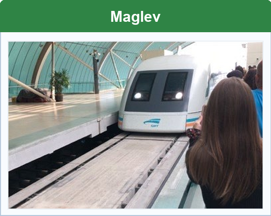
• Magnetic levitation (maglev): High-speed systems that are propelled and guided by electromagnetic forces without physical wheel–rail contact. While maglev does not produce wheel–rail contact stresses, the guideway structure must still resist significant aerodynamic and magnetic forces.

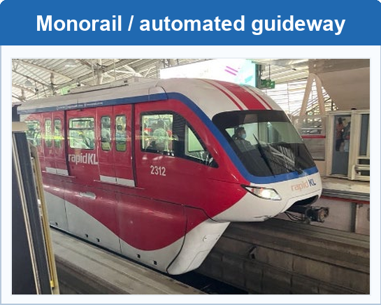
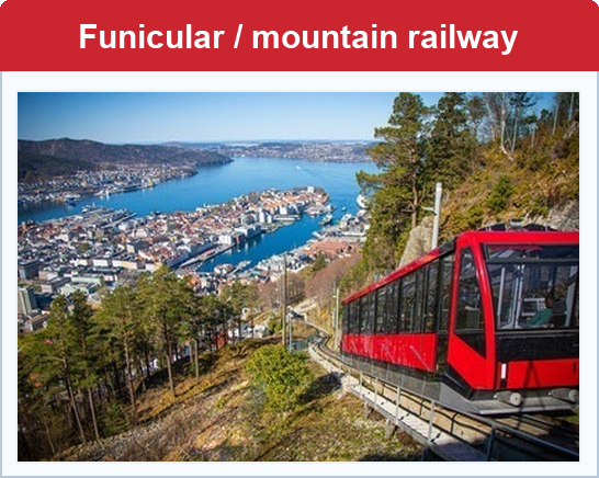
• Other guided systems: Monorails, automated people movers, funiculars, and rack railways are often designed around a dedicated guideway, traction, or braking concept rather than the standard two-rail wheel–rail interface.

Three examples are useful for understanding why specialised railway systems must be treated separately from ordinary two-rail track:

• Monorail and automated guideway systems run on a dedicated beam or guideway. The structural load path is therefore governed by the guideway beam and support columns rather than by rail, sleeper, and ballast behaviour.

• Maglev systems use electromagnetic support, guidance, and propulsion. They do not create wheel–rail contact stresses, but the guideway must carry magnetic, aerodynamic, braking, and vehicle loads.

• Funicular and mountain railway systems are designed for steep gradients. Cable assistance, braking systems, and local guideway geometry become central design features.

The common point in these specialised systems is that the load-transfer mechanism is system-specific rather than governed by the conventional wheel–rail interface.

Figure 1.3 Examples of specialised railway systems.(a) monorail and automated guideway transit; (b) magnetic-levitation railway (maglev); and (c) funicular and mountain railway.

1.3 Wheel Arrangement Classification

The number and arrangement of axles on a locomotive or multiple-unit train set determine how the total vehicle mass is distributed over the track. The wheel arrangement or axle arrangement is therefore a fundamental parameter in any traffic loading analysis.

Three major classification systems are in use worldwide [115, 148]:

1. The AAR system, used in North America for diesel and electric locomotives.

2. The Whyte notation, historically used in North America and Britain for steam locomotives.

3. The UIC classification (also called the German system), used across continental Europe, including Norway.

1.3.1 The UIC Classification System

The UIC classification is administered by the International Union of Railways (UIC) and is standardised in IRS 60650 [115]. Line classification for maintenance purposes follows UIC 714 [169]. The notation is built from the following elements:

• Capital letters denote groups of driven (powered) axles: A = 1 driven axle, B = 2 driven axles, C = 3 driven axles, D = 4 driven axles, and so on.

• Lowercase "o" appended to a capital letter indicates that each axle in the group has its own independent traction motor (e.g. "Bo" = two individually motored driven axles). Without "o", the axles in the group are coupled mechanically.

• Arabic numerals denote groups of non-driven (unpowered) axles: 1 = 1 non-driven axle, 2 = 2 non-driven axles, etc.

• Apostrophe (\('\)) after a letter or numeral indicates that the corresponding axle group is mounted in a pivoting bogie (truck) rather than fixed directly to the main frame.

• Parentheses group letters and numerals that describe the same bogie, and make the apostrophe redundant for indicating bogie mounting.

• Plus sign (+) separates permanently coupled but mechanically independent traction units within the same locomotive or train set.

1.3.2 Common UIC Arrangements

Basic groups (no bogie):

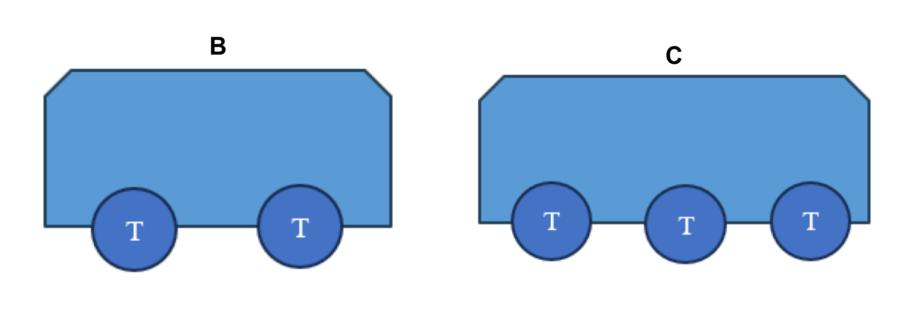
The simplest arrangements mount axles directly on the main frame, as illustrated in Figure 1.4 for "B" (two coupled driven axles) and "C" (three coupled driven axles). These rigid-frame arrangements transmit axle loads directly at fixed positions along the frame. In the sketches used here, \(T\) marks a driven traction axle.

Figure 1.4 Basic UIC driven-axle groups: B has two driven axles and C has three driven axles.

Bogie arrangements:

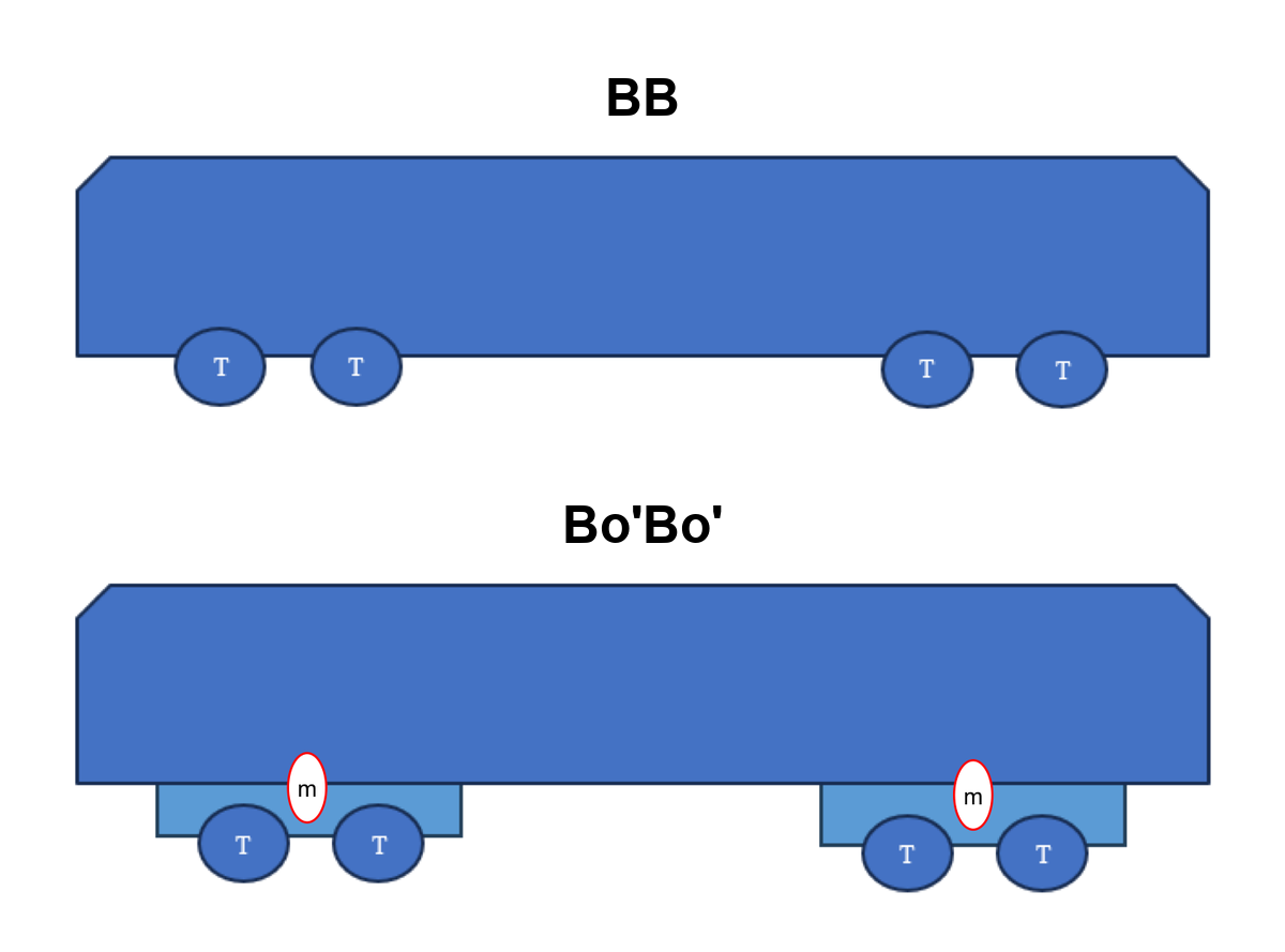
Modern locomotives almost universally use bogies. A bogie is a subframe that carries two or more axles and pivots under the car body, allowing the locomotive to negotiate curves without imposing large lateral forces on the rail. The distinction matters structurally: in Figure 1.5, BB keeps four driven axles fixed to the main frame, whereas Bo'Bo' places the four driven axles in two bogies with individual motors. The red \(m\) in the figure marks the traction motors.

Figure 1.5 Comparison of BB and Bo’Bo’. The apostrophe indicates bogie mounting; “o” indicates individually motored axles.

Longer arrangements:

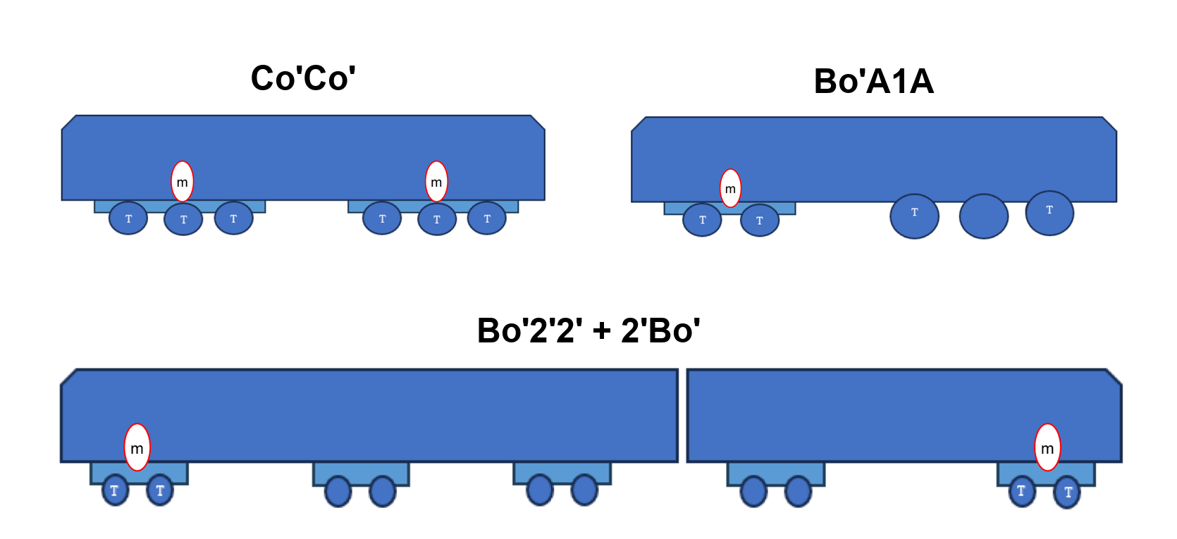
For high-power or heavy-haul applications, six-axle locomotives are common. For this reason, the Co'Co' arrangement in Figure 1.6 is widely used in high-power freight and mixed-traffic service. The same figure also shows two longer axle-arrangement examples: Bo'A1A, where one group contains a non-driven carrying axle, and Bo'2'2' + 2'Bo', where the plus sign separates two permanently coupled but mechanically independent units.

Figure 1.6 Additional UIC examples: Co’Co’, Bo’A1A, and Bo’2’2’ + 2’Bo’. Unlabelled wheels are carrying axles.

The examples above can be read as compact notation rules: letters describe axle groups, apostrophes show bogie mounting, and "o" marks individually motored axles.

Notation	Description
B	2 driven axles, frame-mounted, mechanically coupled
Bo'	2 driven axles, bogie-mounted, individually motored
BB	4 driven axles, frame-mounted
Bo'Bo'	4 driven axles in 2 two-axle bogies, individually motored
Co'Co'	6 driven axles in 2 three-axle bogies, individually motored
Bo'A1A	4 driven axles and 1 non-driven axle; one two-axle driven bogie plus a three-axle group with a carrying axle
Bo'Bo'Bo'	6 driven axles in 3 two-axle bogies (e.g. Alstom PRIMA)
Bo'2'2' + 2'Bo'	4 driven + 6 non-driven axles; two permanently coupled units
(1A)(A1)	4 axles in two bogies, inner two driven; outer two non-driven

Table 1.1 Selected UIC wheel arrangement examples.

Today, the most common wheel arrangements in modern European locomotives are Bo'Bo' (four-axle electric and diesel-electric locomotives for mixed or passenger traffic) and Co'Co' (six-axle high-power or heavy-haul locomotives). The designation determines traction performance and the way loads are distributed onto the track, which directly affects the stresses calculated in Section 1.5.

1.4 Load Distribution Through the Track Structure

This section follows the vertical wheel load from the rail contact point down through the sleepers, ballast, and supporting formation. The main design question is how each layer spreads the load before it reaches the next layer.

1.4.1 Axle Load and Wheel Load

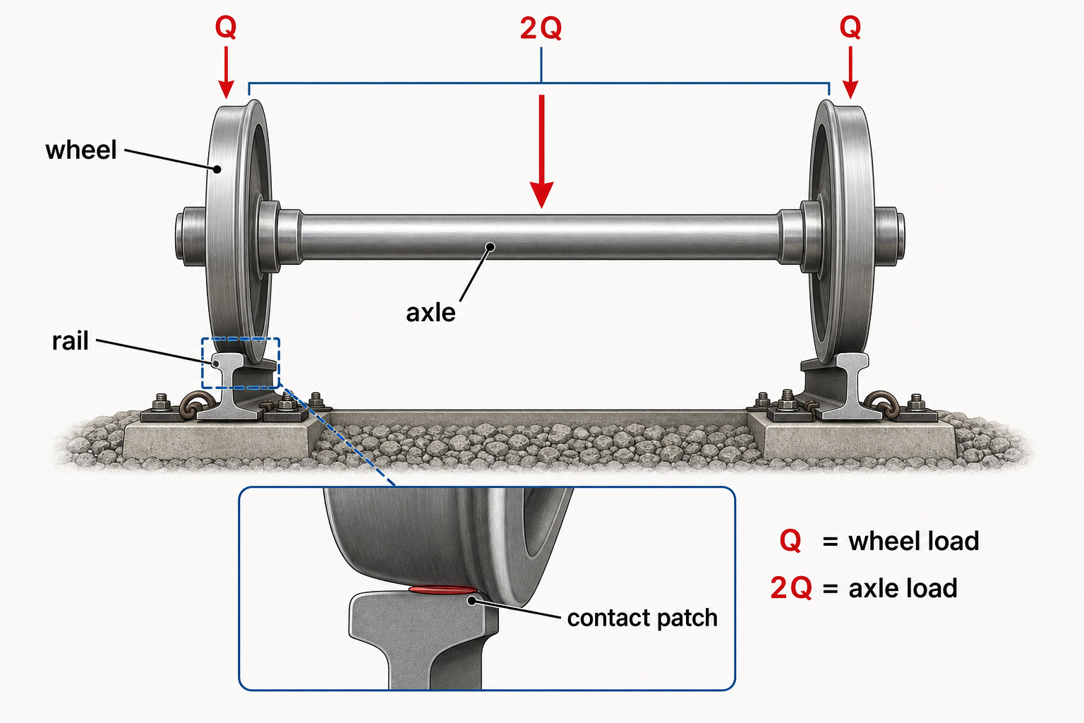
In railway engineering, vehicle loading is standardised in terms of the axle load \(P\), the total vertical force exerted by one complete axle (both wheels combined) on the rails. The wheel load \(Q\) is the share borne by a single wheel. Assuming symmetric loading (which holds on tangent track):

\[ Q = \frac{P}{2} \]

(1.1)

On curved track, centrifugal force and cant deficiency cause the outer wheel to carry a higher load than the inner wheel. This quasi-static load redistribution is discussed in Section 1.6; the wheelset sketch below introduces the two-wheel, two-rail notation used for the load split.

Figure 1.7 Schematic railway wheelset: two wheels mounted on a common axle, rolling on two rails.

The design load is determined by vehicle properties, line classification and operating policy. Typical Norwegian operating cases span from light urban vehicles to route-specific heavy-haul ore traffic.

Train type	Axle load \(P\) [t]	Wheel load \(Q\) [kN]	Notes
Light rail / tram	8–12	39–59	Urban systems
Intercity passenger (EMU)	12–16	59–78	e.g. Flirt, BM73
High-speed passenger	14–17	69–83	Relatively low axle load
Standard freight wagon	22.5	110	European standard
Heavy-haul freight (Ofoten)	30	147	Route-specific ore traffic

Table 1.2 Typical axle loads for different train types (Bane NOR Network Statement 2026 [30]).

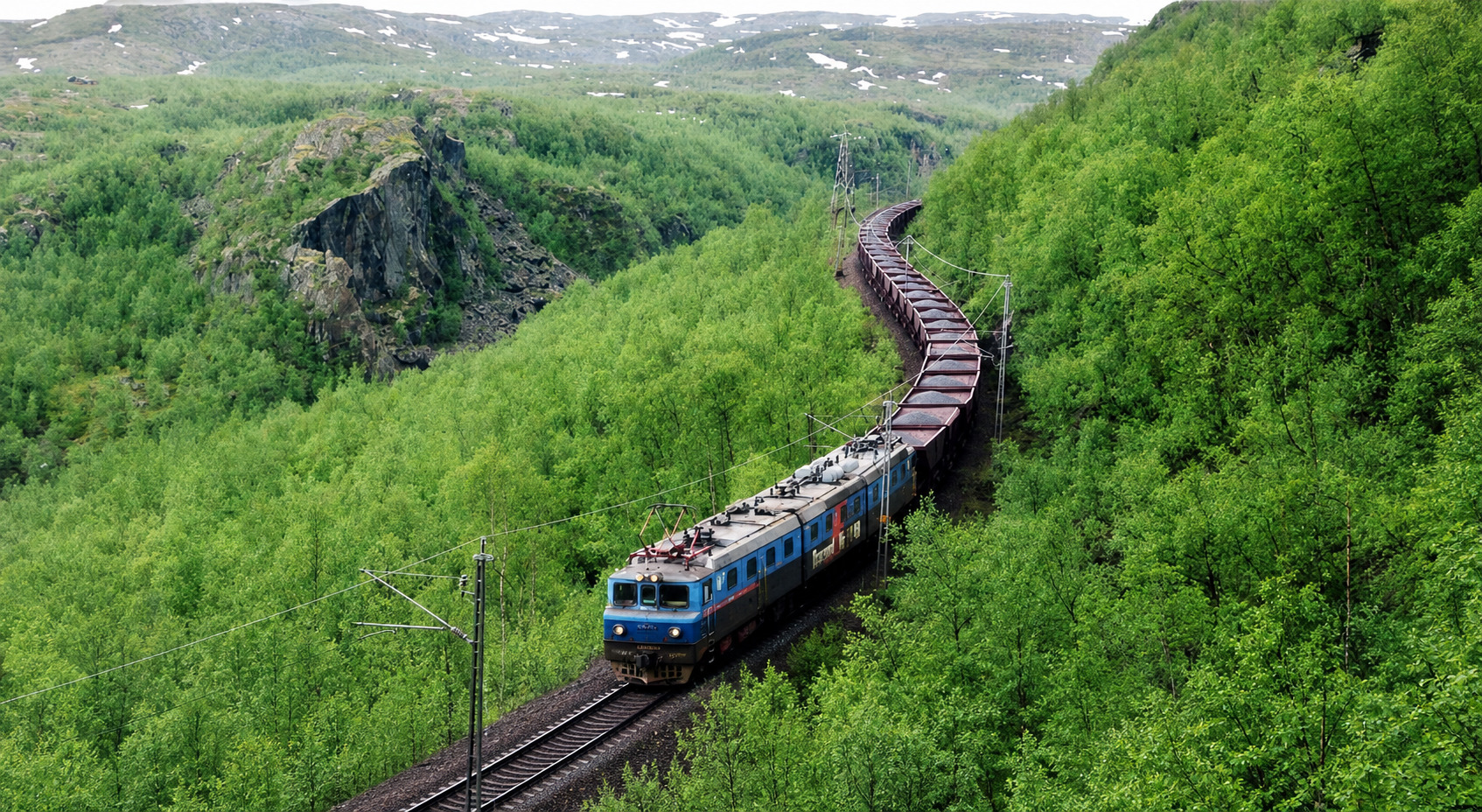
Figure 1.8 shows an Ofotbanen/Malmbanan ore train, a practical example of the upper end of the axle-load range.

Figure 1.8 Heavy-haul ore train on the Ofotbanen/Malmbanan corridor, illustrating route-specific high axle loads.

1.4.2 Components of the Track Structure

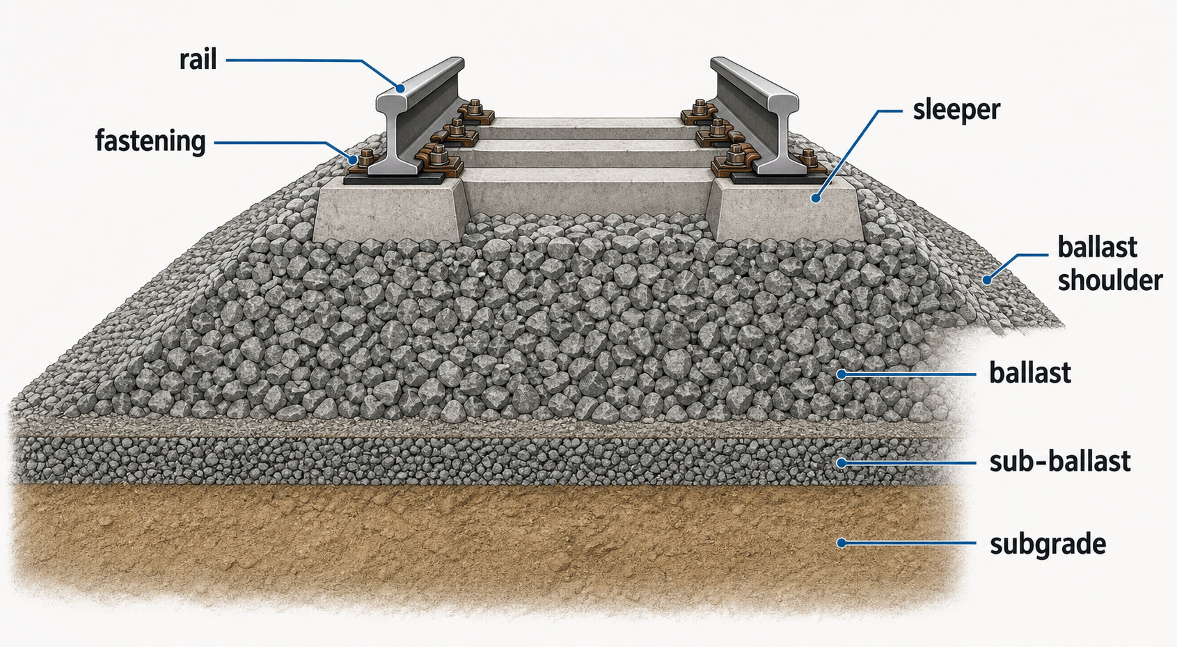
The track structure consists of four main layers, each of which progressively distributes and attenuates the concentrated wheel load before it reaches the subgrade [68, 128, 148]:

1. Rail: Acts as a continuous beam supported on discrete elastic supports (the sleepers). The rail distributes the concentrated wheel load over several neighbouring sleepers, typically three to five in total. The bending stiffness \(EI_x\) of the rail governs how widely the load is spread.

2. Fastenings (rail fixings): Elastic clips, base plates, and screws that connect the rail to the sleeper. They maintain rail inclination (typically 1:20 or 1:40), restrain longitudinal rail movement in continuously welded track, and provide a degree of vertical elasticity [88].

3. Sleepers (crossties or bearers): Transverse elements, typically concrete though historically timber, that transfer rail seat loads to the ballast, maintain track gauge (\(1435\) mm in Norway), and provide lateral resistance against track buckling.

4. Ballast: A layer of crushed hard stone (granite or similar) of controlled particle size (typically 31.5–63 mm in Norway per the technical regulations [10]); aggregate specification is governed by EN 13450 [79]. The ballast distributes the sleeper loads over a wide area of the subgrade at a spreading angle of approximately \(45^\circ\), provides drainage, and allows the track position to be corrected by tamping.

The layered load path described above is shown schematically in Figure 1.9.

Figure 1.9 Schematic ballasted track cross-section showing the principal structural layers.

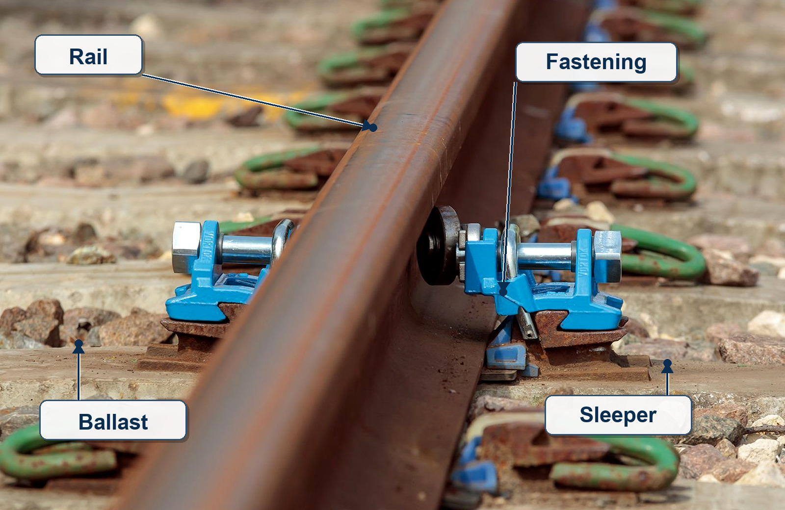
The schematic is complemented by the real track view in Figure 1.10, where the rail, fastening system, sleeper, and ballast can be seen in their usual arrangement.

Figure 1.10 Real ballasted-track components: rail, fastening, sleeper, and ballast.

1.4.3 Load Path and Stress Attenuation

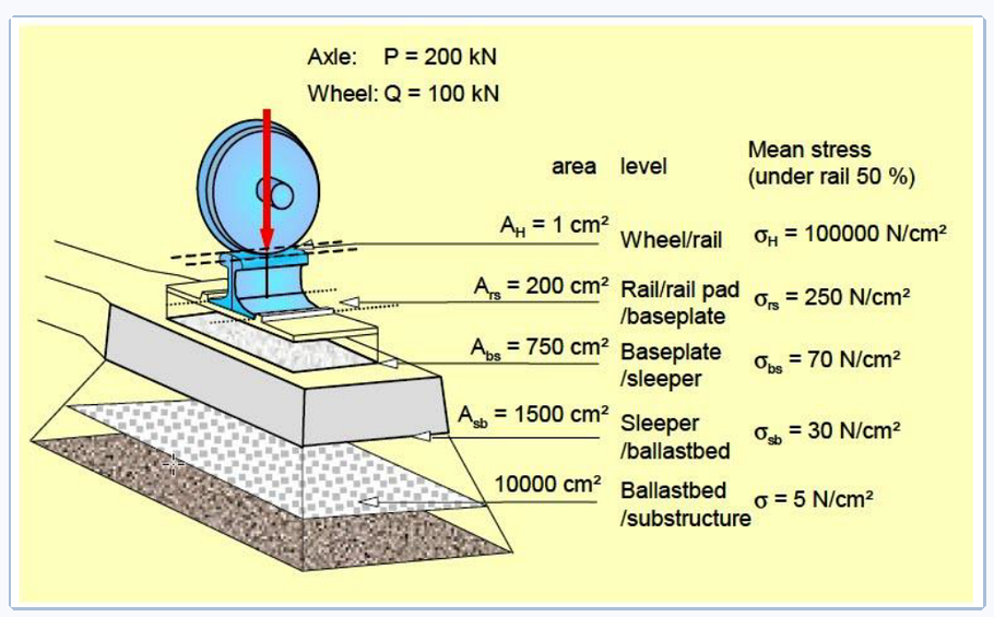
The progressive load spreading from wheel to subgrade is shown in Figure 1.11. Two mechanisms should be distinguished. First, the rail behaves as a beam and distributes one wheel load longitudinally to a group of discrete sleeper reactions, with the largest reaction normally occurring close to the wheel load. Second, each sleeper spreads its reaction downward and outward through the ballast, subballast, and formation. The illustrative percentages in the figure are for a 200 kN axle load (\(Q=100\) kN) and depend on rail stiffness, sleeper spacing, and support stiffness. The wheel–rail contact stress is extremely high: mean design contact pressures are typically several hundred N/mm\(^2\), and local maximum Hertzian pressures may exceed \(1000\) N/mm\(^2\) depending on wheel load, wheel radius, and contact geometry. By the time the load reaches the subgrade surface, it has spread over an area of several square metres, reducing the stress to approximately \(0.05\) N/mm\(^2\) (5 N/cm\(^2\)) [68].

Figure 1.11 Progressive load distribution and stress attenuation through the track structure.

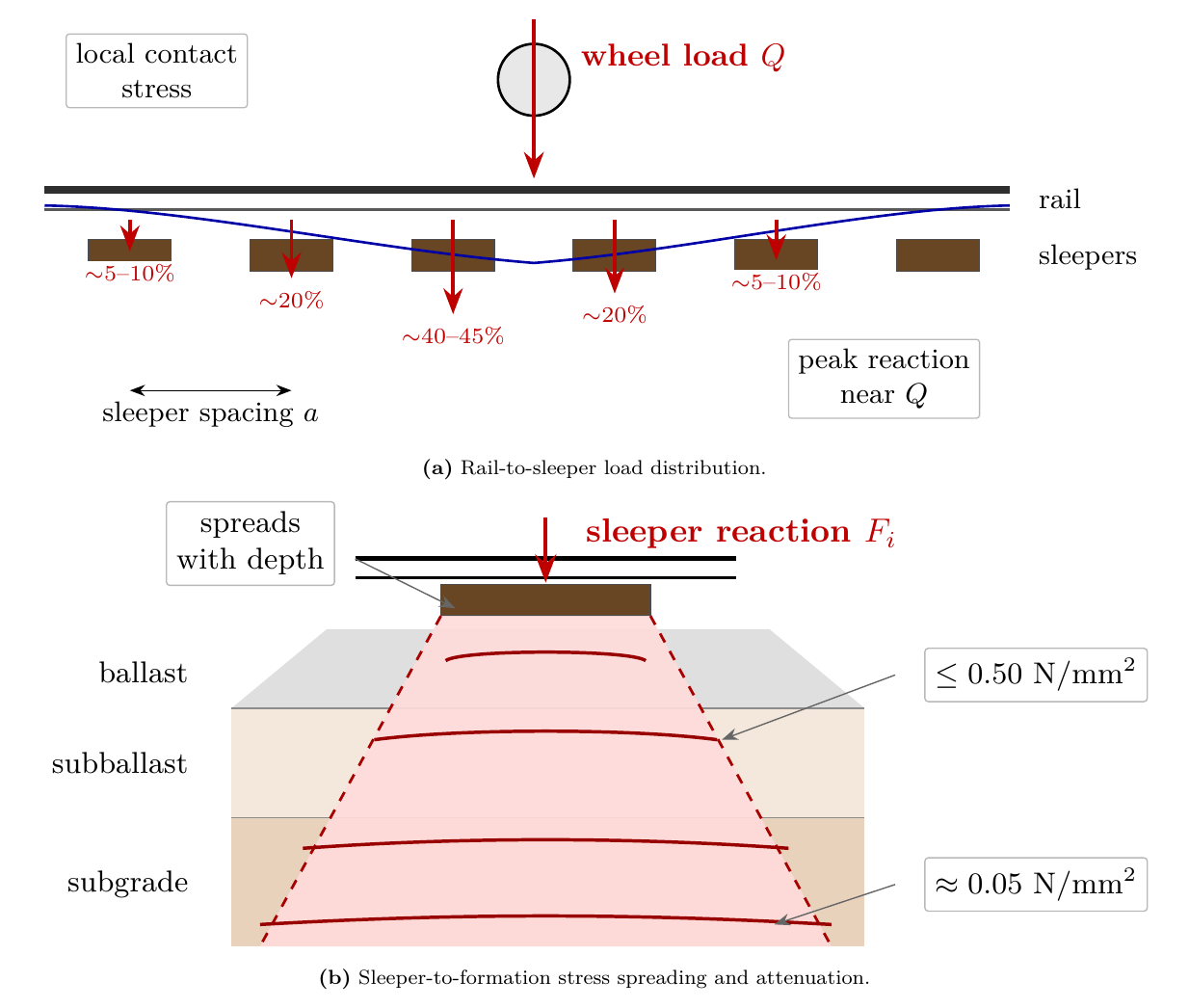
The schematic view in Figure 1.12 presents the same idea using indicative contact areas and stress levels at each interface. It shows why stresses decrease so rapidly through the track structure. The values should be interpreted as order-of-magnitude indicators, not as design limits.

Figure 1.12 Indicative load spreading from wheel–rail contact to the formation.

1.4.4 The Winkler Beam-on-Elastic-Foundation Model

The rail is modelled analytically as an infinitely long beam resting on a continuous elastic foundation, the classical Winkler model [68]. The foundation reaction \(p\) per unit length of rail is assumed proportional to the local deflection \(w\):

\[ p = k \cdot w \]

(1.2)

where \(k\) [N/mm\(^2\)] is the track modulus (foundation stiffness per unit length of rail). In practice, the discrete sleeper supports are represented by the vertical support stiffness of one rail seat (one half-sleeper) \(k_d\) [N/mm] – the spring stiffness of the rail-seat support assembly (sleeper + ballast + subgrade). The relationship between \(k_d\) and the track modulus \(k\) is:

\[ k = \frac{k_d}{a} \]

(1.3)

where \(a\) [mm] is the centre-to-centre sleeper spacing. In the N–mm equations, \(k_d\) must be entered in N/mm. Practical values are often quoted as 20–60 kN/mm (20 000–60 000 N/mm) for good ballasted track and 80–100 kN/mm (80 000–100 000 N/mm) for stiff slab track.

In the schematic model in Figure 1.13, the discrete sleeper supports are represented by an equivalent elastic foundation while the rail carries the wheel load as a bending beam.

Figure 1.13 Rail modelled as an infinite beam on a Winkler elastic foundation, with rail bending stiffness EI_x, vertical support stiffness k_d for one rail seat (one half-sleeper), sleeper spacing a, and characteristic load distribution length L [68].

A related consequence of the beam-on-foundation model is visible in Figure 1.14. The vertical deflection curve \(y(x)\) is controlled by the balance between the rail bending stiffness \(EI_x\) and the support stiffness \(k_d\). Increasing \(EI_x\) makes the rail behave more like a continuous beam, so the load is spread over a longer distance and the separate bogie deflection basins tend to merge. Increasing \(k_d\) reduces the absolute deflection, but it also makes the response more localised beneath each wheelset. For this reason, a stiff track is not automatically a better track; the design aim is an appropriate combination of rail stiffness, sleeper spacing, pad stiffness, ballast support, and formation stiffness.

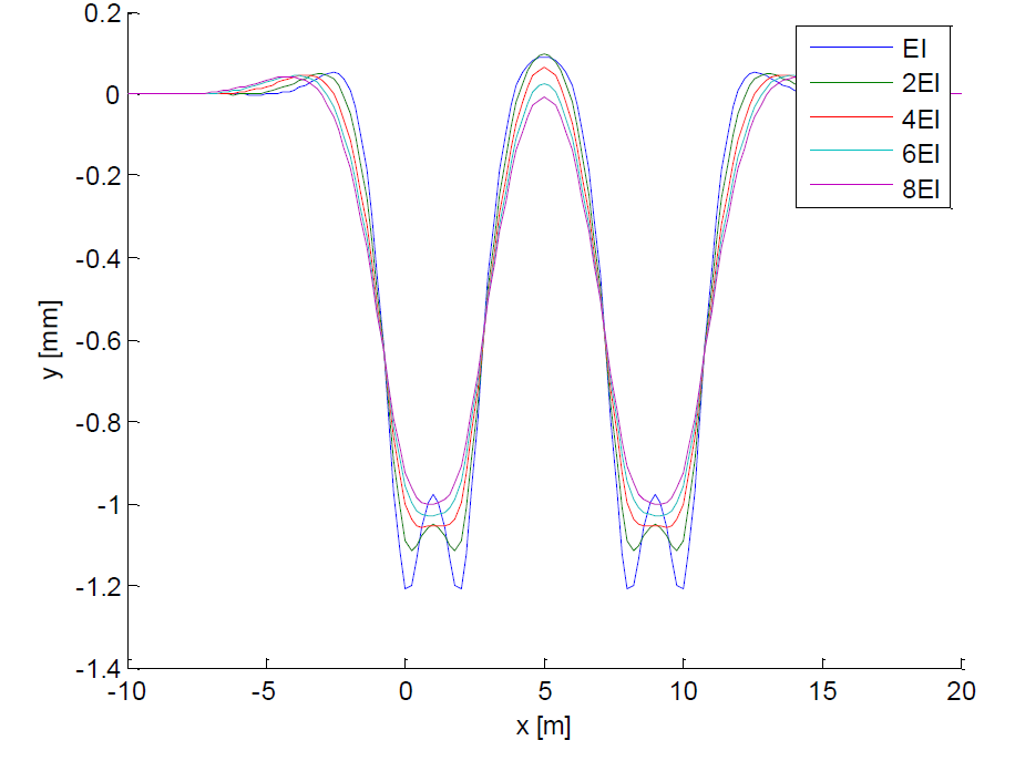
Effect of increasing rail bending stiffness EI_x.

Effect of increasing support stiffness k_d.

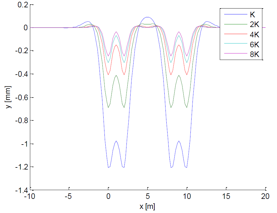
Figure 1.14 Effect of rail and support stiffness on bogie-induced vertical deflection. The curves are qualitative, not design charts.(a) Effect of increasing rail bending stiffness E I x; and (b) Effect of increasing support stiffness k d.

1.5 Static Stress Estimation: the Eisenmann Method

The Eisenmann method [65, 68] provides closed-form equations for the mean stresses and forces in each layer of the track structure under a static wheel load \(Q\). It is based on the Winkler beam model and is the standard analytical tool for preliminary track design in European practice. The method is presented here layer by layer.

The notation used in the stress calculations is collected in Table 1.3 before the layer-by-layer equations are introduced.

Symbol	Unit	Meaning and calculation convention
\(P\)	kN or t	Axle load, i.e. the total load carried by both wheels on one axle. When given in tonnes, convert to force before stress calculations.
\(Q\)	N or kN	Wheel load. In the Eisenmann equations using N and mm, use \(Q\) in N.
\(Q_0\)	kN	Static wheel load expressed in kN for the simplified contact-stress formula.
\(I_x\)	mm\(^4\)	Rail second moment of area about the horizontal neutral axis. The subscript avoids confusion with cant deficiency.
\(D_c\)	mm	Cant deficiency used in the quasi-static curve-load discussion.
\(a\)	mm	Centre-to-centre sleeper spacing.
\(k_d\)	N/mm	Vertical support stiffness for one rail seat (one half-sleeper). Practical values may be quoted in kN/mm; multiply by 1000 before using N–mm equations such as Eq. 1.7.
\(L\)	mm	Characteristic length of the rail beam on elastic foundation.
\(F_0\)	N	Fastening clamping force at one rail seat.
\(A_{rs}\), \(A_{sb}\)	mm\(^2\)	Effective rail–sleeper and sleeper–ballast contact areas. Values given in cm\(^2\) must be multiplied by 100.
\(t\), \(\varphi\)	N/A	Eisenmann confidence factor and track-quality coefficient used in the DAF.

Table 1.3 Notation and calculation units used in this chapter's stress calculations.

1.5.1 Rail Head: Contact Stress

The actual wheel–rail contact has a three-dimensional, approximately elliptical pressure distribution. For a preliminary rail-head check, Eisenmann's simplified two-dimensional model replaces the contact ellipse by a rectangular strip of width \(2s\) and uses the mean contact stress [64, 68, 15]:

\[ q_{\mathrm{mean}} = \sqrt{\frac{\pi E Q}{64(1-\nu^2)\,r\,s}} \]

(1.4)

where:

• \(Q\) = wheel load [N]

• \(E\) = Young's modulus of rail steel = 210 000 N/mm\(^2\)

• \(\nu\) = Poisson's ratio of steel = 0.30

• \(r\) = wheel radius [mm] (typically 430–500 mm for new wheels)

• \(s\) = assumed half-width of the rectangular wheel–rail contact strip [mm]

With \(E=210\,000\) N/mm\(^2\), \(\nu=0.30\), and \(s=6\) mm, the practical Eisenmann relation is [64, 68, 15]:

\[ q_{\mathrm{mean}} = 1374\sqrt{\frac{Q_0}{r}} \quad [\mathrm{N/mm^2}] \]

(1.5)

where \(Q_0\) is the static or quasi-static wheel load in kN and \(r\) is the wheel radius in mm. The coefficient 1374 is unit-specific and includes the assumptions stated above; it is not dimensionless. For a fixed wheel radius, this simplified line-contact model gives \(q_{\mathrm{mean}}\propto\sqrt{Q_0}\). It is distinct from a full Hertz solution for the actual contact ellipse, for which the peak pressure scales with the cube root of the normal load when geometry and material properties remain fixed.

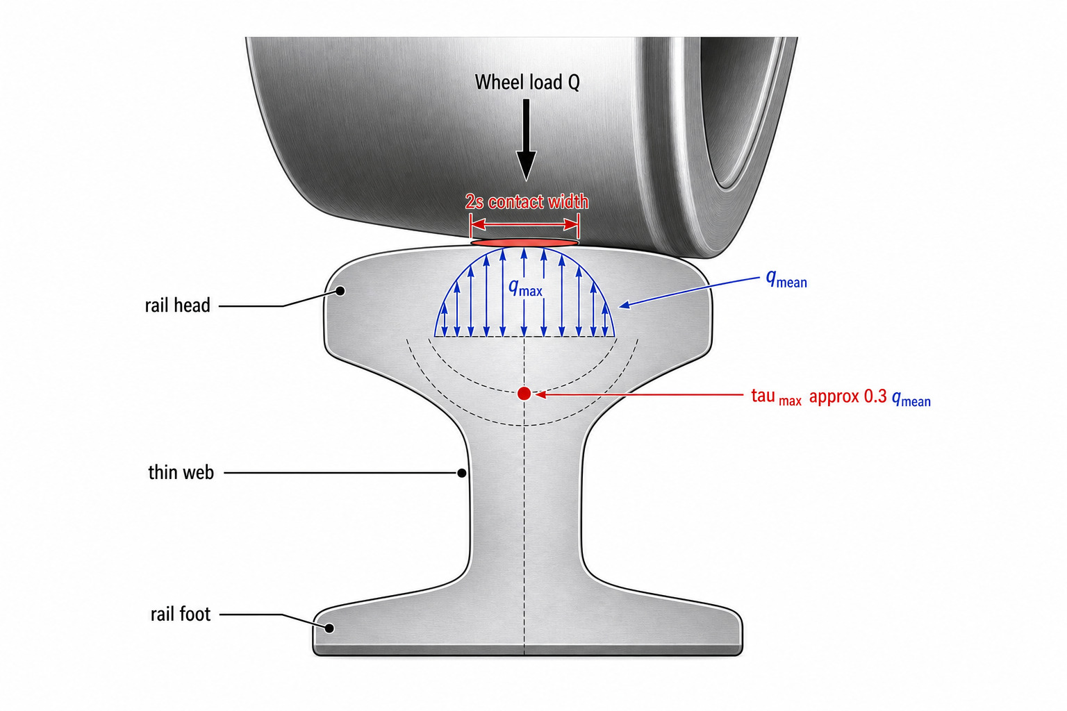
The maximum shear stress occurs below the rail head surface and can contribute to the initiation of rolling contact fatigue (RCF) cracks. In this screening calculation it is approximated as [68]:

\[ \tau_{\max} \approx 0.3\;q_{\mathrm{mean}} \]

(1.6)

at a depth of about 4–6 mm below the running surface.

Equation 1.6 is an approximation within Eisenmann's simplified line-contact model and is used only for the preliminary screening chain in this chapter. It must not be combined with the pressure ratios from a full Hertz ellipse. In the three-dimensional Hertz model, the area-mean pressure is \(\bar p=N/(\pi ab)\) and the peak pressure is \(p_0=3N/(2\pi ab)=1.5\bar p\); neither quantity is identical to Eisenmann's \(q_{\mathrm{mean}}\). The maximum subsurface shear stress and its depth also depend on the ellipse aspect ratio and the traction state. The defect perspective on rolling contact fatigue is introduced in Chapter 4; the full contact model is developed later in Chapter 10.

The stress concentration at the wheel–rail contact is sketched in Figure 1.15, including the contact width and the location of maximum subsurface shear stress.

Figure 1.15 Schematic wheel–rail Hertzian contact stress distribution in the rail head, showing contact width 2s, contact pressure q, and the approximate location of maximum subsurface shear stress.

1.5.2 Rail Foot: Bending Stress

The rail bends under the concentrated wheel load according to the Winkler model. The characteristic length \(L\) is the fundamental parameter of the beam-on-elastic-foundation solution [65]:

\[ L = \sqrt[4]{\frac{4\,E\,I_x\,a}{k_d}} \]

(1.7)

where:

• \(E\) = Young's modulus of rail steel [N/mm\(^2\)]

• \(I_x\) = second moment of area of the rail cross-section about the horizontal neutral axis [mm\(^4\)]

• \(a\) = centre-to-centre sleeper spacing [mm]

• \(k_d\) = vertical support stiffness for one rail seat (one half-sleeper) [N/mm]

The characteristic length \(L\) represents the distance over which the rail distributes the point load: a longer \(L\) means the load is spread over more sleepers, which reduces the peak sleeper force but does not necessarily reduce the rail bending stress. Typical values of \(L\) for ballasted main-line track range from 700–1100 mm.

The mean bending tensile stress at the rail foot centre, the critical section for fatigue, is [65, 68]:

\[ \sigma_{\mathrm{mean}} = \frac{Q \cdot L}{4\,W_{yf}} \]

(1.8)

where \(W_{yf}\) [mm\(^3\)] is the section modulus of the rail cross-section with respect to the bottom fibre (rail foot).

Table 1.4 gives the geometric properties of the two rail profiles most commonly used in Norway. The 60E1 profile (previously designated UIC 60) is the standard for new construction on main lines; UIC 54 is found on older sections and secondary lines.

Profile	\(A\) [cm\(^2\)]	\(I_x\) [cm\(^4\)]	\(W_{yf}\) [cm\(^3\)]	\(W_{yh}\) [cm\(^3\)]	Mass [kg/m]
UIC 54	69.34	2 346	235	268	54.43
60E1 (UIC 60)	76.86	3 055	335	378	60.34

Table 1.4 Geometric properties of rail profiles used in Norway (Bane NOR technical regulations, Overbygning/Prosjektering/Sporkonstruksjoner [10]).

1.5.3 Sleeper: Rail Seat Force and Interface Stress

The mean vertical force on the most heavily loaded sleeper beneath a single wheel is estimated from the loaded length of rail [68]:

\[ F_{\mathrm{mean}} \approx \frac{Q \cdot a}{2\,L} \]

(1.9)

where \(a\) is the sleeper spacing and \(2L\) is the effective load-distribution length. The vertical rail-seat support stiffness \(k_d\) controls the characteristic length \(L\) in the Winkler model, but it is not multiplied directly into this force expression.

The mean contact pressure at the rail–sleeper interface (or rail seat pressure) must account for the pre-stress introduced by the fastening clamping force \(F_0\):

\[ \sigma_{rs} = \frac{F_0 + F_{\mathrm{mean}}}{A_{rs}} \]

(1.10)

where:

• \(F_0\) = total fastening clamping force at the rail seat [N] (both clips, one rail)

• \(A_{rs}\) = effective contact area at the rail seat [mm\(^2\)] (with base plate: plate area; without: rail foot area)

The allowable rail–sleeper interface pressures according to the technical regulations [10] are:

• Softwood (pine) sleepers: \(\sigma_{rs} \leq 1.0\)–\(1.5\) N/mm\(^2\)

• Hardwood (oak) sleepers: \(\sigma_{rs} \leq 1.5\)–\(2.5\) N/mm\(^2\)

• Prestressed concrete sleepers: \(\sigma_{rs} \leq 4.0\) N/mm\(^2\)

Concrete sleepers are the standard on Norwegian main lines; timber sleepers are retained on some low-traffic secondary lines and sidings [130].

1.5.4 Ballast: Sleeper–Ballast Interface Stress

The load is distributed from the sleeper to the ballast over the effective bearing area \(A_{sb}\) of one half of the sleeper. The mean sleeper–ballast contact stress is [68, 128]:

\[ \sigma_{sb} = \frac{F_{\mathrm{mean}}}{A_{sb}} \]

(1.11)

The allowable ballast contact pressure in Bane NOR technical regulations [10] is:

\[ \sigma_{sb} \leq 0.50\ \mathrm{N/mm^2} \]

(1.12)

This limit governs the minimum required sleeper bearing area \(A_{sb}\) for a given load and track stiffness. Equation 1.11 shows that \(\sigma_{sb}\) can be reduced by:

• Increasing \(A_{sb}\): using wider or longer concrete sleepers (e.g. twin-block sleepers instead of monoblock, or B70 instead of B60 type).

• Decreasing \(F_{\mathrm{mean}}\): reducing sleeper spacing \(a\) or increasing the characteristic length \(L\) (for example by increasing rail bending stiffness or reducing support stiffness, provided deflection and settlement limits are still satisfied).

Worked example setup.

A section of conventional main-line track is checked against Bane NOR technical regulation stress limits at \(v = 120\) km/h. The following data are used in the static calculation below and in the later dynamic continuation.

Parameter	Value
Static wheel load	\(Q = 100\ \mathrm{kN}\)
Rail profile	UIC 54: \(I_x = 2346\times10^4\ \mathrm{mm^4}\), \(W_{yf} = 235\times10^3\ \mathrm{mm^3}\), \(r = 500\ \mathrm{mm}\)
Vertical support stiffness, one rail seat	\(k_d = 12\ \mathrm{kN/mm}=12{,}000\ \mathrm{N/mm}\)
Sleeper spacing	\(a = 600\ \mathrm{mm}\)
Fastening clamping force	\(F_0 = 20\ \mathrm{kN}\) (per rail, per rail seat)
Rail–sleeper contact area	\(A_{rs} = 550\ \mathrm{cm^2}\) (concrete sleeper with base plate)
Sleeper–ballast contact area	\(A_{sb} = 837\ \mathrm{cm^2}\) (half sleeper bearing area)
Material	\(E = 210{,}000\ \mathrm{N/mm^2}\), \(\nu = 0.3\)
Track quality	Normal (\(\varphi = 0.2\))

Worked example: static stress checks.

Using the data given in the worked example setup, the static wheel–rail contact stress is

\[ \begin{aligned} q_{\mathrm{mean}} &= 1374\sqrt{\frac{Q_0}{r}},\\ &= 1374\sqrt{\frac{100}{500}},\\ &= 614.5\ \mathrm{N/mm^2}. \end{aligned} \]

and the approximate maximum subsurface shear stress is \(\tau_{\max}\approx0.3q_{\mathrm{mean}}=184.3\) N/mm\(^2\).

The characteristic length is

\[ L = \sqrt[4]{\frac{4 \times 210{,}000 \times 2346\times10^4 \times 600}{12{,}000}} = 996\ \mathrm{mm}. \]

The rail-foot bending stress and the most heavily loaded sleeper force are

\[ \begin{aligned} \sigma_{\mathrm{mean}} &= \frac{100{,}000 \times 996}{4 \times 235{,}000} = 105.9\ \mathrm{N/mm^2},\\ F_{\mathrm{mean}} &= \frac{100{,}000 \times 600}{2 \times 996} = 30.1\ \mathrm{kN}. \end{aligned} \]

The interface stresses are then

\[ \sigma_{rs} = \frac{20{,}000 + 30{,}100}{550 \times 100} = 0.91\ \mathrm{N/mm^2} \leq 4.0\ \mathrm{N/mm^2}, \]

\[ \sigma_{sb} = \frac{30{,}100}{837 \times 100} = 0.360\ \mathrm{N/mm^2} \leq 0.50\ \mathrm{N/mm^2}. \]

Both static interface checks are within the technical regulation limits.

1.6 Dynamic Traffic Loading

Static axle load is only the starting point for track design. Speed, curvature, wind, and track irregularities add dynamic effects that can govern local stresses and maintenance needs.

1.6.1 Quasi-Static Forces: Curves and Cross-Winds

When a train negotiates a horizontal curve at speed \(v\) [km/h] with radius \(R\) [m], the centrifugal acceleration acts outward on both the vehicle and its contents. If the track is superelevated (canted) by a height \(h_a\) [mm], the centrifugal effect is partially balanced. The cant deficiency \(D_c\) [mm] quantifies the uncompensated centrifugal effect [68]:

\[ \begin{aligned} D_c &= h_{\mathrm{ideal}} - h_a,\\ h_{\mathrm{ideal}} &= \frac{11.8\,v^2}{R}\ \text{[mm]}. \end{aligned} \]

(1.13)

Cant deficiency first produces an uncompensated lateral inertial force. That force then produces a roll moment about the wheel–rail contact line, increasing the vertical wheel load on the outer rail and reducing it on the inner rail. A dimensionally consistent estimate is:

\[ Y_c = G\,\frac{D_c}{b_c} \]

(1.14)

\[ \Delta Q = \frac{Y_c h_d + Y_w h_w}{b_g} \]

(1.15)

where \(Y_c\) = curve-induced lateral inertial force per axle [kN], \(G\) = axle weight [kN], \(D_c\) = cant deficiency [mm], \(b_c\) = effective cant base (approximately 1500 mm), \(\Delta Q\) = increase in vertical wheel load on the outer rail [kN], \(Y_w\) = lateral wind force per axle [kN], \(h_d\) = height of centre of gravity above rail [m], \(h_w\) = height of wind-force resultant above rail [m], and \(b_g\) = lateral distance between wheel–rail contact points [m]. Thus:

\[ \begin{aligned} Q_{\mathrm{outer}} &\approx \frac{G}{2} + \Delta Q,\\ Q_{\mathrm{inner}} &\approx \frac{G}{2} - \Delta Q. \end{aligned} \]

(1.16)

The centrifugal contribution to the outer wheel load typically represents 10–25% of the static wheel load, depending on speed, cant deficiency, vehicle centre-of-gravity height, and gauge geometry.

1.6.2 Track Irregularities and Vehicle Defects

In reality, track geometry is never perfectly smooth. Geometric irregularities, including corrugation, rail joints, transition zones, switches and crossings, and vehicle defects such as wheel flats and out-of-round wheels, all generate additional dynamic forces above the static value [130, 91]. Local defects such as these can convert an otherwise smooth wheel passage into an impact-like load event.

Figure 1.16 Defects that can amplify dynamic wheel loads: (a) wheel-flat or tread damage; (b) rail corrugation; and (c) a squat or other local rail-head defect.

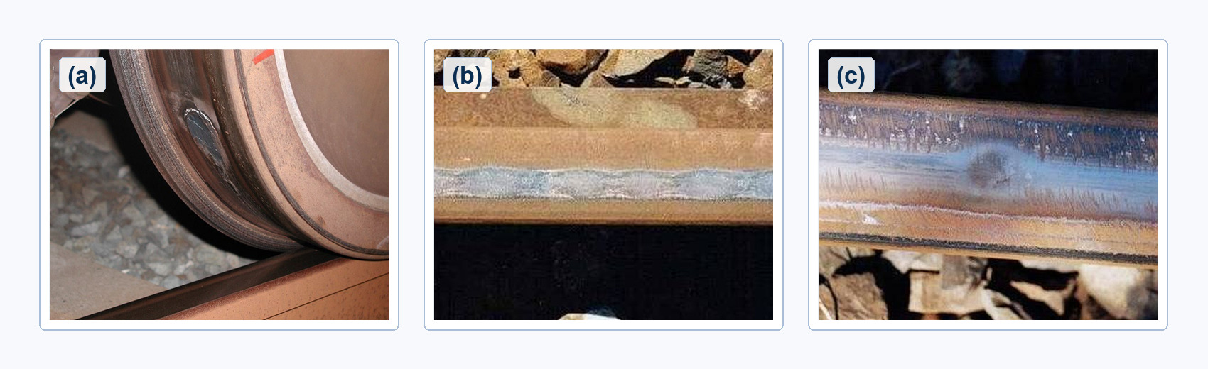
Dynamic forces are inherently stochastic: they vary from one axle passage to the next, depend on the specific combination of track and vehicle condition, and cannot be predicted deterministically [117]. A probabilistic design approach is therefore adopted, characterised by the Dynamic Amplification Factor (DAF).

1.6.3 The Dynamic Amplification Factor (DAF)

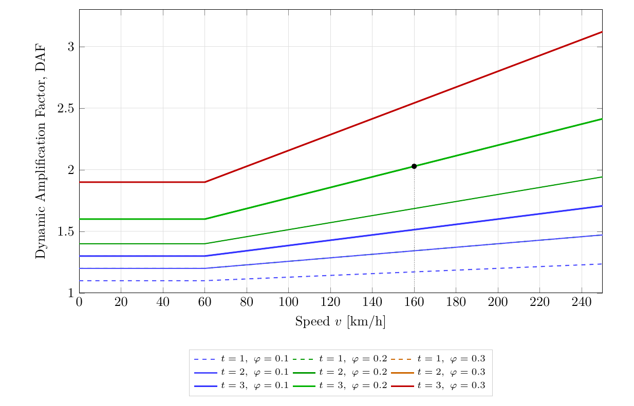
The Eisenmann DAF [65, 68] amplifies the static stresses and forces to obtain the design (maximum expected) values. It is defined as:

\[ \mathrm{DAF} = 1 + t\,\varphi \qquad \text{for } v < 60\ \mathrm{km/h} \]

(1.17)

\[ \mathrm{DAF} = 1 + t\,\varphi\!\left(1 + \frac{v - 60}{140}\right) \qquad \text{for } 60 \leq v \leq 200\ \mathrm{km/h} \]

(1.18)

where:

• \(v\) = train speed [km/h]

• \(\varphi\) = track quality coefficient (see Table 1.5)

• \(t\) = confidence factor, equal to the number of standard deviations above the mean (Table 1.5)

The statistical basis of the DAF is important to understand. The axle load is not increased because the vehicle becomes heavier; rather, the measured wheel force fluctuates around the static value as the vehicle and track interact dynamically. The dynamic load increment is assumed to be normally distributed with mean zero and standard deviation \(\varphi \cdot Q_{\mathrm{static}} \cdot (1 + (v-60)/140)\). By choosing \(t = 1, 2, 3\), the designer selects the 84th, 97.7th, or 99.87th percentile of the load distribution, respectively. For rail bending stresses, fastenings, and supports, \(t = 3\) is standard. For ballast and subgrade, \(t = 2\) is considered adequate [68].

Track quality	Description	\(\boldsymbol{\varphi}\)	Recommended use
Good	New or well-maintained; regular tamping	0.1	High-speed lines
Normal	Standard maintenance cycle	0.2	Mixed-traffic main lines
Poor	Deferred maintenance; high defect density	0.3	Conservative design

Table 1.5 Track quality coefficient \(\varphi\) and confidence factor \(t\) (Eisenmann DAF formula [65, 68]). Confidence factors: \(t = 3\) for rail bending, fastenings, and supports (99.87th percentile); \(t = 2\) for ballast and subgrade (97.7th percentile).

The speed dependence is plotted in Figure 1.17 for three track quality classes and three confidence levels. At 160 km/h with normal track quality (\(\varphi = 0.2\)) and \(t = 3\):

\[ \mathrm{DAF} = 1 + 3\times0.2\times\!\left(1+\frac{160-60}{140}\right) = 1 + 0.6\times1.714 = 2.03. \]

Figure 1.17 Eisenmann DAF for φ ∈ {0.1, 0.2, 0.3} and t ∈ {1, 2, 3}. The black marker shows the example at v = 160 km/h, normal track quality and DAF = 2.03.

1.6.4 Design Stresses Including DAF

The maximum (characteristic) stresses and forces used for the track-component checks below are obtained by applying the appropriate DAF to the static wheel load. For quantities that are linear in wheel load, this is equivalent to multiplying the static value by the DAF.

The local rail-head contact check is treated separately. Its complete simplified relation is \(q_{\mathrm{mean}}=1374\sqrt{Q_0/r}\); the square root contains the full ratio \(Q_0/r\). For a given wheel radius it is proportional to the square root of the wheel load, but the practical Eisenmann check uses the static or quasi-static wheel force; the \(t=3\) track-component DAF is not automatically inserted into this formula [68, 15]. A dynamic wheel–rail contact assessment must instead start from an independently determined dynamic wheel force and an appropriate contact model.

Table 1.6 therefore distinguishes the separate rail-head contact check from the DAF-amplified track-component responses.

Component / interface	Static value	Dynamic design value	Typical check
Wheel–rail contact	\(q_{\mathrm{mean}} = 1374\sqrt{Q_0/r}\)	Separate contact assessment; no DAF applied here	Can contribute to rail-head fatigue and RCF risk
Rail foot bending	\(\sigma_{\mathrm{mean}} = QL/(4W_{yf})\)	\(\sigma_d = \mathrm{DAF}_{t=3}\,\sigma_{\mathrm{mean}}\)	Tensile stress at rail foot; fatigue / fracture margin
Rail seat force	\(F_{\mathrm{mean}} \approx Qa/(2L)\)	\(F_d = \mathrm{DAF}_{t=3}\,F_{\mathrm{mean}}\)	Pad, fastening, and sleeper rail-seat demand
Rail–sleeper pressure	\(\sigma_{rs}=(F_0+F_{\mathrm{mean}})/A_{rs}\)	\(\sigma_{rs,d}=(F_0+F_d)/A_{rs}\)	\(\leq 4.0\) N/mm\(^2\) for concrete sleepers
Sleeper–ballast pressure	\(\sigma_{sb}=F_{\mathrm{mean}}/A_{sb}\)	\(\sigma_{sb,d}=\mathrm{DAF}_{t=2}\,\sigma_{sb}\)	\(\leq 0.50\) N/mm\(^2\) at the ballast contact
Top of subgrade	Estimated from load spreading through ballast/subballast	Use \(\mathrm{DAF}_{t=2}\) on the transmitted vertical stress	Compare with subgrade bearing capacity and settlement criteria

Table 1.6 Summary of the separate rail-head contact check and the DAF-based track-component calculations (after [64, 65, 68, 15]).

Worked example: dynamic design values.

For normal track quality, \(\varphi=0.2\). Although the design speed is 120 km/h, the low-speed case \(v=20\) km/h is also shown to make the DAF multiplication transparent:

\[ \begin{aligned} \mathrm{DAF}_{t=3}(20) &= 1 + 3\times0.2 = 1.60,\\ \mathrm{DAF}_{t=2}(20) &= 1 + 2\times0.2 = 1.40. \end{aligned} \]

At \(v=120\) km/h,

\[ \mathrm{DAF}_{t=3}(120) = 1 + 3\times0.2\times\!\left(1+\frac{120-60}{140}\right) = 1.857, \]

\[ \mathrm{DAF}_{t=2}(120) = 1 + 2\times0.2\times\!\left(1+\frac{120-60}{140}\right) = 1.571. \]

The simplified rail-head contact check remains the separate static or quasi-static value \(q_{\mathrm{mean}}=614.5\) N/mm\(^2\) calculated above. It is not re-amplified by the track-component DAF in this example. If a dynamic contact assessment is required, the dynamic wheel force must be established separately before an appropriate contact model is applied. Rail-foot bending stress is linear in wheel load, so it is multiplied directly by \(\mathrm{DAF}_{t=3}\):

\[ \begin{aligned} \sigma_d(20) &= 1.60\times105.9 = 169.4\ \mathrm{N/mm^2},\\ \sigma_d(120) &= 1.857\times105.9 = 196.7\ \mathrm{N/mm^2}. \end{aligned} \]

For the rail–sleeper interface, only \(F_{\mathrm{mean}}\) is amplified; the fastening clamping force \(F_0\) remains static:

\[ \begin{aligned} \sigma_{rs,d}(20) &= \frac{20{,}000 + 48{,}200}{550\times100} = 1.24\ \mathrm{N/mm^2},\\ \sigma_{rs,d}(120) &= \frac{20{,}000 + 55{,}900}{550\times100} = 1.38\ \mathrm{N/mm^2}. \end{aligned} \]

For the sleeper–ballast interface, the ballast check uses \(\mathrm{DAF}_{t=2}\):

\[ \begin{aligned} \sigma_{sb,d}(20) &= 1.40\times0.360 = 0.504\ \mathrm{N/mm^2},\\ \sigma_{sb,d}(120) &= 1.571\times0.360 \approx 0.565\ \mathrm{N/mm^2}. \end{aligned} \]

Quantity	Static	\(v = 20\) km/h \((t=3:\ 1.60;\ t=2:\ 1.40)\)	\(v = 120\) km/h \((t=3:\ 1.86;\ t=2:\ 1.57)\)	Limit
Rail head contact stress \(q\) [N/mm\(^2\)]	614.5	–	–	Separate check
Rail foot bending stress \(\sigma\) [N/mm\(^2\)]	105.9	169.4	196.7	N/A
Rail–sleeper pressure \(\sigma_{rs}\) [N/mm\(^2\)]	0.91	1.24	1.38	\(\leq 4.0\)
Sleeper–ballast pressure \(\sigma_{sb}\) [N/mm\(^2\)]	0.360	0.504	0.565	\(\leq 0.50\)

Table 1.7 Separate static contact check and DAF-amplified track-component values for the worked example.

The sleeper–ballast pressure marginally exceeds the 0.50 N/mm\(^2\) limit already at 20 km/h (\(0.504\) N/mm\(^2\)) and exceeds it more clearly at 120 km/h, so the ballast interface controls this example. At 120 km/h, the required half-sleeper bearing area is approximately 947 cm\(^2\) if all other assumptions are unchanged. The margin can be improved by increasing the sleeper bearing area, reducing sleeper spacing and recomputing \(L\) and \(F_{\mathrm{mean}}\), or specifying better track quality.

1.7 Wheel-Group Rail Stress Checks

The Eisenmann calculations above treat the wheel load and the most heavily loaded sleeper as the starting point for preliminary stress checks. For bogie vehicles, neighbouring wheels on the same rail can also influence the bending moment under a reference wheel. A compact Winkler–Zimmermann influence-line check is useful when a rail-foot stress check must include axle spacing explicitly [68, 62, 65].

For a wheel at distance \(x\) from the reference wheel, the influence coefficient is

\[ \begin{aligned} \xi &= \frac{x}{L},\\ \mu &= e^{-\xi}(\cos\xi - \sin\xi). \end{aligned} \]

(1.19)

where \(L\) is the characteristic length of the rail on its support. For the reference wheel, \(x=0\) and \(\mu=1\). Let \(N_\mathrm{w}\) be the number of wheels on the same rail included in the check. The wheel-group factor is defined as

\[ S_\mu = \sum_{i=1}^{N_\mathrm{w}} \mu_i. \]

After the dynamic design wheel load has been selected, the maximum rail bending moment may be written

\[ M_\mathrm{max} = \frac{Q_\mathrm{design} L}{4}S_\mu, \]

(1.20)

where \(Q_\mathrm{design}\) is the design wheel load on one rail and \(L\) is inserted in metres when \(M_\mathrm{max}\) is required in kNm. The corresponding rail-foot tensile stress is

\[ \sigma_\mathrm{foot} = \frac{M_\mathrm{max}\,[\mathrm{kNm}]\cdot10^6}{W_{yf}\,[\mathrm{mm}^3]} \quad [\mathrm{N/mm^2}]. \]

(1.21)

The following compact examples show how the influence coefficients are used in practice.

Worked example: two-axle bogie.

Assume a preliminary rail check with characteristic length \(L=0.80\) m, design wheel load \(Q_\mathrm{design}=140\) kN, rail-foot section modulus \(W_{yf}=335\cdot10^3\) mm\(^3\), and a second wheel on the same rail at axle spacing \(x=2.0\) m. The reference wheel has \(\mu_1=1\). For the second wheel,

\[ \begin{aligned} \xi_2&=\frac{x}{L}=\frac{2.0}{0.80}=2.50,\\ \mu_2&=e^{-2.50}(\cos 2.50-\sin 2.50)=-0.115. \end{aligned} \]

Thus

\[ S_\mu = \sum_{i=1}^{2}\mu_i = \mu_1+\mu_2 = 1-0.115 = 0.885. \]

The maximum bending moment and rail-foot stress are then

\[ M_\mathrm{max} =\frac{140\cdot0.80}{4}\cdot0.885 =24.8\,\mathrm{kNm}, \]

\[ \sigma_\mathrm{foot} =\frac{24.8\cdot10^6}{335\cdot10^3} =74\,\mathrm{N/mm^2}. \]

In this example the neighbouring wheel lies in a negative part of the influence line, so it slightly reduces the reference-wheel bending moment. This is possible because the rail behaves as a beam on an elastic foundation, not as a simply supported beam.

Quick sensitivity: closer neighbouring wheel.

If the same neighbouring wheel were much closer, for example \(x=0.40\) m with the same \(L=0.80\) m, then

\[ \begin{aligned} \xi_2&=0.50,\\ \mu_2&=e^{-0.50}(\cos0.50-\sin0.50)=0.241, \end{aligned} \]

so

\[ S_\mu=\sum_{i=1}^{2}\mu_i=1+0.241=1.241. \]

The same design wheel load would give

\[ \begin{aligned} M_\mathrm{max} &=\frac{140\cdot0.80}{4}\cdot1.241 =34.8\,\mathrm{kNm},\\ \sigma_\mathrm{foot} &=104\,\mathrm{N/mm^2}. \end{aligned} \]

The spacing relative to \(L\) determines the interaction factor, so neighbouring wheels cannot be added as full wheel loads.

This check is not a replacement for the layer-by-layer Eisenmann method above; it is an additional rail-bending check for cases where neighbouring wheel spacing and rail section properties must be made explicit.

1.7.1 Classical Continuous-Support Parameters

Older Norwegian and German design practice describes the rail support not by a discrete rail-seat stiffness \(k_d\) and sleeper spacing \(a\), but by a ballast coefficient \(C_b\) (N/cm\(^3\)) acting on an equivalent continuously supported rail width \(b\). The two descriptions are exchangeable: the continuous foundation stiffness per unit length is \(C_b\,b\), and the characteristic length becomes

\[ L=\sqrt[4]{\frac{4\,E\,I_x}{b\,C_b}}, \]

(1.22)

which replaces the discrete form of Eq. 1.7 when \(C_b\) and \(b\) are the given support data. Three further conventions belong to this classical method and are used when older data sets or exam-style tasks are formulated in it:

• Wheel-force displacement correction. A supplement of \(0.1\,Q_\mathrm{static}\) is added to the static wheel force before the rail check, representing load transfer between the wheels of an axle from cant, curving and load eccentricity.

• Classical speed factor. The dynamic design wheel load is written \(Q_\mathrm{design}=Q\,(1+n\,\varphi_v)\), where the speed factor is \(\varphi_v = 1 + 0.5\,(v-60)/80\) for \(60<v\leq140\) km/h (and \(\varphi_v=1\) below 60 km/h), and \(n\) describes the track condition: \(n=0.1\) for very good, \(n=0.2\) for good, and \(n=0.25\) for other or mediocre track. Note carefully that the speed factor \(\varphi_v\) is not the same quantity as the Eisenmann track-quality factor \(\varphi\) used earlier in this chapter; the subscript \(v\) is used here to keep the two symbols apart.

• Minimum wheel radius and corresponding diameter. The classical wheel-size criterion limits the contact stress under a given wheel force by requiring the minimum radius defined immediately below.

The minimum wheel radius is

\[ r_\mathrm{min}=1.67\cdot10^{6}\,Q\left(\frac{\nu_s}{\sigma_\mathrm{break}}\right)^{2}, \]

(1.23)

where \(Q\) is in kN, the rail tensile strength \(\sigma_\mathrm{break}\) is in N/mm\(^2\), \(r_\mathrm{min}\) is in mm, and \(\nu_s\) is a wheel-load utilisation factor that depends on the line category (\(\nu_s = 1.2\) is a representative value for a second-order freight line). The corresponding minimum wheel diameter is \(D_\mathrm{min}=2r_\mathrm{min}\); any specified wheel diameter \(D\) must be compared with \(D_\mathrm{min}\), not directly with \(r_\mathrm{min}\). These conventions allow classical support descriptions to be interpreted consistently when translating between line-load and discrete rail-seat (half-sleeper) support-stiffness data.

1.8 Bane NOR Superstructure Classes

Bane NOR classifies its track into superstructure classes that define the maximum permitted axle load as a function of speed [32, 169]. Each line section is assigned a superstructure class based on the rail profile, sleeper type and spacing, ballast depth, and subgrade condition. The class is an important input to route availability, but permitted operation may also be restricted by bridges, substructure condition, track geometry, local speed restrictions, and vehicle-specific approvals.

The compact class overview in Table 1.8 links these infrastructure classes to the axle-load and speed limits used later in the compendium. The values are taken from Bane NOR's Operativt regelverk, SJN 2.18.1, updated 15 August 2025 [32].

Class	Passenger coaches		EMU/DMU sets
	Axle load [t]	v [km/h]	Axle load [t]	v [km/h]
a	16	90	16	90
b	18	100	18	100
c	18	160	20.5/18	130/160
c+	18	160	20.5	160
d	18	230	20.5/20/18/17	160/200/250/300
Ofotbanen	18	130	20.5	130

Class	Freight and work vehicles
	Axle load [t]	v [km/h]	vbogie [km/h]
a	22.5/16.5	30/70	30/70
b	22.5/20.5/18	30/70/80	30/70/80
c	22.5/20.5/18	80/90/100	90/100/110
c+	241/22.5/20.5/18	50/90/100/110	50/100/110/120
d	25/22.5/18	70/100/110	70/120/120
Ofotbanen	31/22.5	50/702	50/70

Table 1.8 Bane NOR superstructure classes from Operativt regelverk/SJN 2.18.1 (updated 15 August 2025) [32]. Separate limits are needed because passenger coaches, multiple units, and freight/work vehicles have different axle spacing and dynamic behaviour.

¹The 24 t entry applies only on the Nordlandsbanen section from Guldsmedvik (km 499.517) to Ørtfjell (km 534.630). ²The maximum speed for empty ore wagons is 60 km/h.

In the freight/work-vehicle table, \(v_\mathrm{bogie}\) is the maximum speed for bogie vehicles approved under EN 14363. Slash-separated axle loads and speeds pair positionally within each row; for example, the first axle-load entry is paired with the first speed entry. The 24 t entry for class c+ applies only to Nordlandsbanen, Guldsmedvik–Ørtfjell. For Ofotbanen, empty ore wagons are limited to 60 km/h although the table shows 70 km/h for the corresponding class entry. The Ofotbanen row should be read as a route-specific class table, not as a blanket permission for every vehicle. Iron-ore trains typically operate at 30 t axle load, whereas 31 t is the infrastructure/special-rule ceiling shown in the class table. Any use of that ceiling remains subject to the current Network Statement, vehicle approval, bridge and substructure restrictions, and local speed conditions [30, 10].

Regarding rail steel quality, Bane NOR technical regulations [10] requires higher-strength, head-hardened or premium grades for high-axle-load lines:

• For axle loads \(\leq 22.5\) t: Grade R260 (minimum tensile strength 880 N/mm\(^2\)) is standard.

• For axle loads \(> 24\) t: Bane NOR lists premium grades such as R350HT, R370CrHT, R400HT, or R400 UHC XR, independent of curve radius.

• Grade R200 (minimum 680 N/mm\(^2\)) is permitted only on low-speed, low-traffic lines.

Rail profile selection is linked to superstructure class: 60E1 is standard for classes c, c+, and d; UIC 54 may be used for classes a and b [85]. Ofotbanen's heavy axle-load operation requires premium rail steel and route-specific approval; the permitted operational axle load must respect substructure, bridge, and geometry restrictions as well as the superstructure class [165, 10].

1.9 Chapter Summary

Traffic demand. The loads acting on the track are determined first by the railway service: urban railways, conventional mixed-traffic lines, heavy-haul corridors and specialised railways place different requirements on axle load, speed, braking, acceleration and traffic repetition. Vehicle notation such as Bo'Bo' and Co'Co' therefore describes the vehicle and tells the engineer how the weight and traction forces are distributed between axles and bogies.

Load path. A vertical wheel load starts as a concentrated contact force at the rail head, but it is spread progressively through the rail, sleeper, ballast, subballast and formation. The stresses become lower with depth because the loaded area increases, but this does not make the lower layers unimportant. Weak ballast or formation changes the support stiffness and can increase rail bending, sleeper pressure and long-term settlement.

Dynamic effects. Static axle load and wheel load provide the basic design quantities, but real railway loading includes quasi-static forces from curvature, cant deficiency and wind, and dynamic forces from speed, vehicle defects and track irregularities. The dynamic amplification factor expresses this practical reality: the same nominal axle load may become a more severe design action on rough track, at high speed or when wheel and rail defects introduce impact loading.

System compatibility. The rail section, sleeper spacing, ballast support and substructure capacity must be consistent with the traffic class using the line. Heavy axle-load routes such as Ofotbanen illustrate that approval cannot be based on the superstructure alone; bridges, formation, curve geometry, rail steel, maintenance condition and route specific restrictions all influence whether a given traffic load can be accepted safely.

Assignments

Assignment 1: Locomotive wheel arrangement and static load

A locomotive is classified as Co'Co'. Explain fully what each symbol in this designation means. Calculate the static wheel load if the total locomotive mass is 90 t and the load is equally distributed over all six axles. Compare this with a Bo'Bo' locomotive of the same total mass, and state which vehicle is less demanding for a line with strict axle-load limits.

Assignment 2: UIC wheel-arrangement diagrams

Draw the following UIC wheel arrangements. Vehicle bodies and bogies may be represented by simple rectangles, wheelsets by circles, and driven wheelsets by the letter \(T\). Use a vertical line to show the separation between permanently coupled vehicle units. For each arrangement, state the total number of axles and the number of driven axles.

(a) Bo'Bo'

(b) Co'Co'

(c) Bo'2'Bo'

(d) 2'Bo' + 2'2'

(e) Bo'2'2'2'2' + 2'2'Bo'

(f) Bo'2'2'Bo' + 2'2'Bo'

(g) Bo'(1+1)(1+1)(1+1)Bo'

Assignment 3: Track response under wheel load

A track section is loaded by a static wheel load \(Q = 150\) kN. The track uses UIC 54 rail with \(I_x = 2346\times10^4\) mm\(^4\) and \(W_{yf} = 235\times10^3\) mm\(^3\). Other data are: \(k_d = 12\) kN/mm \(=12{,}000\) N/mm, \(a = 600\) mm, \(F_0 = 20\) kN, \(A_{rs} = 550\) cm\(^2\), \(A_{sb} = 837\) cm\(^2\), \(E = 210{,}000\) N/mm\(^2\), \(\nu = 0.30\), wheel radius \(r = 500\) mm, and wheel–rail contact width \(2s = 20\) mm.

(a) Calculate the characteristic length \(L\).

(b) Calculate the static wheel–rail contact stress \(q_{\mathrm{mean}}\) and the approximate maximum subsurface shear stress \(\tau_{\max}\).

(c) Calculate the static rail-foot bending stress \(\sigma_{\mathrm{mean}}\).

(d) Calculate the static rail–sleeper pressure \(\sigma_{rs}\) and sleeper–ballast pressure \(\sigma_{sb}\).

(e) Check \(\sigma_{rs}\) and \(\sigma_{sb}\) against the technical regulation limits used in this chapter, and state which interface controls the design.

Assignment 4: Dynamic load and speed effect

Use the same track and wheel load as in Assignment 3. Assume good track quality (\(\varphi = 0.10\)).

(a) Calculate the dynamic rail-foot bending stress and wheel-load contribution to rail-seat pressure at \(v=20\) km/h and \(v=120\) km/h using \(t=3\); use \(t=2\) for sleeper–ballast pressure. The fastening clamping force \(F_0\) is not multiplied by DAF. Report the Eisenmann wheel–rail screening value separately using the stated static or quasi-static load.

(b) Prepare a spreadsheet table or plot for speeds from 0 to 200 km/h in 20 km/h intervals. Include the three track quality classes \(\varphi = 0.10\), \(0.20\), and \(0.30\), and confidence factors \(t = 1\), \(2\), and \(3\). Show how speed, track quality, and confidence level affect rail-foot bending stress, rail–sleeper pressure, and sleeper–ballast pressure.

(c) Briefly explain why the Eisenmann contact screening is kept separate from the DAF-based component curves and why a detailed peak-pressure assessment requires a full Hertz/contact model.

Assignment 5: Ofotbanen axle-load approval check

Ofotbanen is operated under route-specific high-axle-load conditions. A maintenance team is considering using a conventional 25-t-axle-load tamping machine on an Ofotbanen section.

(a) Explain qualitatively how the DAF changes when the machine travels at 60 km/h on a line with poor track quality (\(\varphi = 0.30\), \(t = 3\)) compared with a well-maintained line (\(\varphi = 0.10\), \(t = 3\)).

(b) Using the Eisenmann formula, calculate the dynamic wheel load for both cases and compare them with the static wheel load.

(c) Explain whether the 25-t machine may be used safely and under what conditions.

(d) Propose track monitoring criteria (deformation, stress) that the maintenance team should apply after tamping operations on the high- axle-load section.

Assignment 6: Wheel-group rail stress check

Check the following rail design scenario using the classical continuous-support conventions of Section 1.7.1. Calculate the axle load; calculate \(r_\mathrm{min}\) and then \(D_\mathrm{min}=2r_\mathrm{min}\); compare the actual wheel diameter \(D\) with \(D_\mathrm{min}\); and calculate the maximum rail bending moment and rail-foot tensile stress. Then comment on any design adjustments that may be needed.

The case is an "other" second-order freight line maintained by a newly purchased tamping machine, with the following properties:

• Corroded long welded 60E1 rail, \(I_x = 3055\) cm\(^4\) and \(W_{yf}=335\) cm\(^3\)

• Rail elastic modulus \(E = 21\cdot10^6\) N/cm\(^2\)

• Width of equivalent continuously supported rail, \(b = 50\) cm

• Sleeper spacing \(a = 55\) cm

• Rail tensile strength \(\sigma_\mathrm{break}=900\) N/mm\(^2\); wheel-load factor \(\nu_s = 1.2\)

• Ballast coefficient \(C_b = 110\) N/cm\(^3\)

• Static wheel force \(Q_\mathrm{static}=100\) kN

• Wheel-force displacement correction \(=0.1Q_\mathrm{static}\)

• Track condition: other / mediocre

• Vehicle speed: 100 km/h

• Two-axle bogie with wheelbase \(x=2.0\) m

• Wheel diameter \(D=92\) cm