12

Railway Noise and Vibration

Brief video explanation Watch video

An optional AI-generated overview. Use the written chapter as the authoritative source.

0:00/–:––

CC 0.75× 1× 1.25× 1.5× 2×

In this chapter

12.1 Introduction

Railway transportation is one of the most energy-efficient and environmentally friendly forms of land transport. However, it is also a significant source of noise and vibration for people living and working near rail lines. As rail networks expand and train speeds increase, managing the acoustic and vibratory impact of railways has become a central challenge in both infrastructure planning and rolling stock design [158, 68].

This chapter covers the principal sources of railway noise, the mechanisms by which vibration propagates from the track into the ground and into adjacent buildings, the measurement methods and regulatory limits used to quantify and control noise exposure, and the mitigation measures available to the track engineer, infrastructure manager, and vehicle designer.

Rail is a high-capacity, energy-efficient form of land transport, but increasing traffic and development near lines, stations and depots can expose more people to noise and vibration. Noise calculations therefore influence land-use planning, the location of new buildings and the design of railway upgrades. Planning the railway and its surroundings together can avoid problems that are difficult to solve once both are built.

Noise from railways affects the health and quality of life of large numbers of people. WHO’s evidence review [174] considers several health outcomes of transport noise, with evidence assessed separately by noise source and outcome. Relevant health concerns include:

• Sleep disturbance and sleep deprivation (from pass-by events at night).

• Cardiovascular health effects: WHO reports associations between environmental noise exposure and ischaemic heart disease and hypertension. The evidence should be interpreted for the relevant noise source and health outcome; no railway-specific disease threshold is inferred here. See WHO’s 2022 environmental-noise overview [204].

• Annoyance and reduced cognitive performance in children, particularly for schools adjacent to busy lines.

Vibration from railways is a separate but related problem. Ground-borne vibration can cause:

• Physical discomfort and possible sleep disturbance for building occupants (perceptible vibration at frequencies 1–80 Hz).

• Disturbance of sensitive equipment such as electron microscopes, lithography machines, and laboratory balances, even where vibration is too low to damage the equipment.

• Possible structural effects in unusually sensitive buildings or severe exposure conditions. Perceptible vibration does not by itself establish a risk of damage; structural assessment requires separate criteria from human comfort.

• Re-radiated noise ("rumble") in buildings, where vibration of walls, floors and ceilings converts to low-frequency airborne sound.

Norwegian railway projects are assessed under several overlapping noise regimes: planning guidance for new land use and new infrastructure, action limits for existing sources, and European requirements for strategic noise mapping. The important practical point is to keep these contexts separate rather than treating one limit value as a universal railway-noise requirement [123, 131, 95].

Health-burden studies can express the combined consequences in disability-adjusted life years (DALYs), combining years of life lost with years lived with disability. This is a population-health measure, not an acoustic indicator or a compliance limit for one dwelling. The lecture introduces it to explain why exposure, annoyance and health outcomes matter alongside measured decibel levels [223].

Assessment context	Main question	Principal Norwegian or European framework
Planning	How should a new railway, an upgrade or noise-sensitive development be located and designed?	T-1442 and associated planning and building requirements.
Existing sources and buildings	Does the existing exposure require mapping or remedial action?	Chapter 5 of the Pollution Control Regulations (Forurensningsforskriften).
Strategic mapping	Where is the population exposed across major railway corridors and agglomerations?	Environmental Noise Directive 2002/49/EC and its assessment methods.

Table 12.1 Assessment contexts for railway noise and vibration.

These contexts are developed in Section 12.5. A source-emission requirement for a train and an exposure criterion at a dwelling also answer different questions.

12.2 Sound, Propagation and Perception

12.2.1 Source, Path and Receiver

A noise or vibration problem can be traced through three connected parts. The source is the vehicle and track: rolling contact, engines, auxiliary equipment, impacts and friction-induced vibration generate the excitation. The path includes sound propagation through air, vibration and sound radiation from the track, and wave propagation through the ground. The receiver is the person, building or sensitive equipment where the effect is assessed [223].

Figure 12.1 separates the source, transmission path and receiver. Use that chain to locate a mitigation measure: reducing excitation at the track, interrupting propagation and protecting a building address different parts of the same problem.

Figure 12.1 Source, transmission path and receiver. From Torbjørn Ursin’s lecture [223].

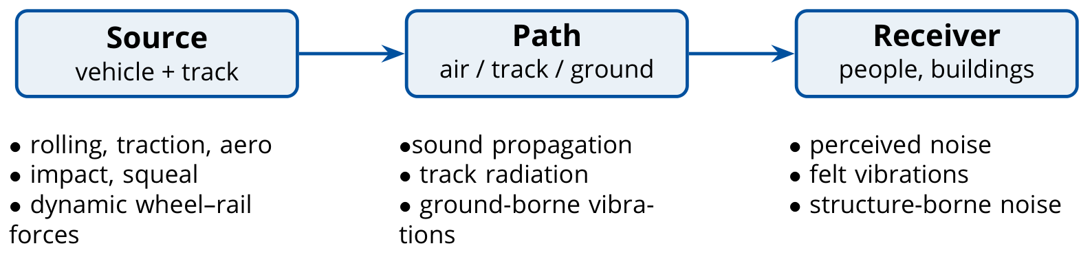
The same contact force can produce both airborne sound and ground-borne vibration. A nearby resident may hear direct railway noise, feel vibration and hear sound re-radiated by the building. Identifying the dominant route is essential: a barrier interrupts airborne propagation but cannot stop vibration travelling through the foundations. Conversely, a softer track support may reduce transmitted vibration while increasing sound radiation from the rail.

12.2.2 Frequency Weighting and Annoyance

Human hearing covers roughly 20 Hz to 20 kHz, with greatest sensitivity commonly around 1–5 kHz. The limits vary between listeners and with sound level. Frequency weighting modifies a measured spectrum before its contributions are combined into one level. A-weighting strongly attenuates low-frequency sound; C-weighting is flatter over much of the audible range and can help describe low-frequency content when the assessment method calls for it [223].

The weighting curves in Figure 12.2 show why the same low-frequency spectrum can produce different A- and C-weighted levels. Compare the low-frequency corrections before treating two reported decibel values as directly comparable.

Figure 12.2 A- and C-weighting across frequency. From Torbjørn Ursin’s lecture [223].

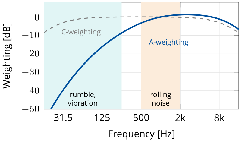
A-weighting is a standardised filter, not a complete model of perception. A tonal fan, corrugated rail or squealing wheel can be more noticeable and annoying than a broadband sound with the same A-weighted level. Impulsive events such as wheel-flat impacts and crossing passages also require attention to their time pattern. The chosen indicator should therefore be interpreted together with the spectrum, duration, repetition and character of the sound. Reporting dB(C) can supplement an assessment, but does not replace a prescribed dB(A) criterion.

12.3 Sources of Railway Noise

Railway noise can be divided into several distinct source types based on the physical mechanism of sound generation. The dominant source changes with speed: traction noise is important at low speed and standstill, rolling noise dominates at ordinary main-line speeds, and aerodynamic noise becomes increasingly important on high-speed lines.

Figure 12.3 compares how the source contributions change with speed. The dominant source can change across the operating range, so a measure aimed at rolling noise need not address aerodynamic or traction noise to the same extent.

Figure 12.3 Indicative speed dependence of railway noise sources. From Torbjørn Ursin’s lecture [223].

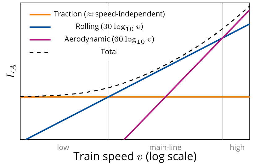
The balance between noise sources does not define universal crossover speeds. Vehicle design, power demand, wheel and rail condition, track support and measurement position all affect the balance. Individual events such as impacts, curve squeal and warning horns must be considered separately [223].

12.3.1 Rolling Noise

Rolling noise is the dominant noise source at speeds above approximately 50–60 km/h for conventional diesel and electric trains, and above about 80 km/h for freight trains. It arises from the combined roughness of the wheel and rail surfaces [158]. The contact mechanics behind this excitation are developed in Chapter 10, while corrugation and roughness were introduced earlier as track defects in Chapter 4.

As the wheel rolls over the rail, micro-scale surface irregularities on both the wheel tread and the rail running surface excite vibrations in the wheel and rail. These vibrating surfaces radiate sound to the surrounding air.

The key parameters governing rolling noise are:

• Wheel and rail roughness: measured as surface height spectra \(L_r(\lambda)\) over wavelengths \(\lambda\) of 3–1000 mm.

• Contact filter: the contact patch acts as a spatial filter, averaging roughness over its dimensions and attenuating contributions at wavelengths shorter than the contact patch length.

• Structural dynamics: the wheel's resonances (typically 800–5000 Hz for the major radiating modes) and the rail's pinned–pinned resonance (typically 800–1200 Hz) amplify roughness excitation near these frequencies [158].

The practical mechanism is the wheel–rail contact itself: surface condition, contact dynamics, and structural vibration combine to determine how much sound is radiated. Torbjørn Ursin’s TWINS diagram below shows the connection from roughness to radiated sound.

The lecture gives an equivalent rolling-noise source-height range of approximately −0.05 to 0.5 m relative to the top of rail. An equivalent source height represents distributed sound radiation in a particular prediction model; it is not the physical height of one component or a universal setting for every calculation [223].

From Surface Roughness to Sound Radiation

The TWINS modelling chain makes the connection between surface condition and received sound explicit. Wheel and rail roughness are combined, the finite contact patch filters that input, the coupled wheel–rail system produces vibration responses, and the wheel, rail and sleeper radiate sound. Propagation then determines the contribution at the receiver. These are distinct stages, so an improvement at one stage does not guarantee an equal reduction in the total received level [223].

Follow Figure 12.4 from wheel and rail roughness through contact excitation to vibration and sound radiation. The chain distinguishes the geometric input from the vehicle and track responses that turn it into airborne noise.

Figure 12.4 From wheel and rail roughness to sound radiation in TWINS. From Torbjørn Ursin’s lecture, after Thompson’s TWINS model [223].

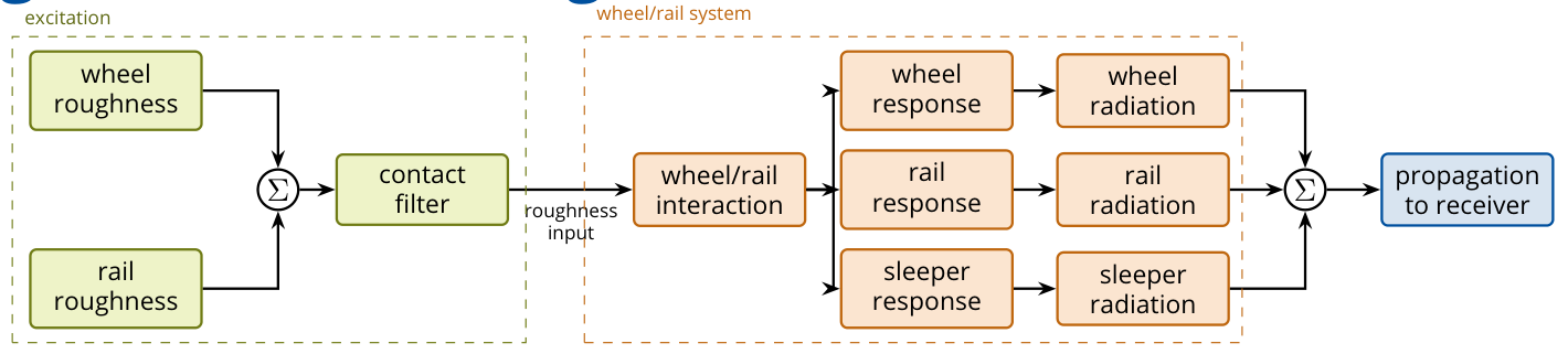
For statistically independent wheel and rail roughness in the same wavelength band and using the same reference, their squared roughness contributions add:

\[ L_{r,\mathrm{comb}}=10\log_{10}\!\left(10^{L_{r,w}/10}+10^{L_{r,r}/10}\right). \]

The rougher surface dominates the combined input. Smoothing an already smooth wheel therefore provides limited benefit if the rail is strongly corrugated, and grinding a smooth rail cannot compensate for very rough wheels. This explains why wheel and rail maintenance should be considered together.

Track decay rate (TDR) describes the spatial decay of rail vibration, in dB/m. A low decay rate means that vibration extends along a longer rail length, increasing the potential radiating length. Rail-pad stiffness, damping and added rail dampers affect this response. TDR is a property of the vibrating track; it is different from the attenuation of airborne sound between track and receiver.

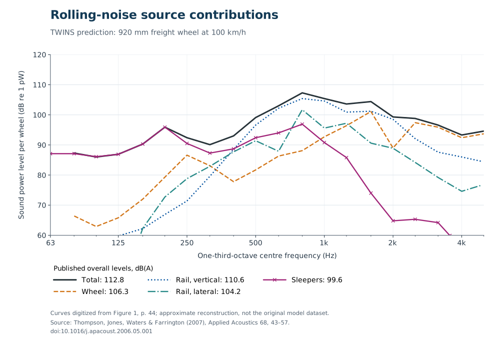
Figure 12.5 uses a documented model example from Thompson et al. [241]: a 920 mm freight wheel at 100 km/h, cast-iron tread-braked wheel roughness, 60E1/UIC60 rail, monobloc concrete sleepers and rail pads with a stiffness of 200 MN/m. The reported per-wheel overall sound-power levels are 112.8 dB(A) in total, 106.3 for the wheel, 110.6 for vertical rail motion, 104.2 for lateral rail motion and 99.6 for the sleeper. These are modelled source sound-power levels referenced to 1 pW, not sound-pressure levels at a dwelling or universal contribution shares. The plotted curves are reconstructed from the published figure; the overall levels in the legend are the values reported by the authors.

Ursin’s lecture [223], slide 14, quotes a separate example with about 99.8 dB(A) for the track and 97.5 dB(A) for the wheel, attributed to Vincent et al. [238] through Nielsen’s NBIU material. That original numerical case has not been independently matched to a publicly available full-text figure, so it is kept separate from the verified example plotted here.

Figure 12.5 Modelled sound-power spectra for a 920 mm freight wheel at 100 km/h. Replotted from Thompson et al. [241].

Speed Dependence

The sound level increases approximately as \(30\log_{10}(v/v_0)\), i.e., by about 9 dB for each doubling of speed.

Worked example.

If the speed of a train increases from 120 to 160 km/h, the rolling-noise increase is

\[ \Delta L_A = 30\log_{10}\!\left(\frac{160}{120}\right) = 3.7\,\text{dB}. \]

This is a large change acoustically: a few decibels can decide whether a mitigation measure is needed.

The lecture also reports an Austrian monitoring example, discussed through UIC and J. Nielsen’s lecture material, with speed coefficients around 29–34. These comparisons help explain the common coefficient of 30, while retaining the distinction between a measured range and a universal law.

Ursin’s lecture includes an unpublished Norwegian measurement example comprising 72 pass-bys of type 74/75 FLIRT electric multiple units at four sites, with the microphone 7.5 m from the track and 1.2 m high. A pooled fit of pass-by equivalent levels gives a speed coefficient \(N=32.1\) dB per decade, with a reported 95% confidence interval of 30.0–34.1 and \(R^2=0.93\), in a relation of the form

\[ L_{Aeq}(v)=L_{Aeq}(v_0)+N\log_{10}(v/v_0). \]

Figure 12.6 plots the measured pass-bys behind the fitted speed relation. The spread around the fit and the range of measured speeds are essential to interpreting the coefficient; the fitted line is not a universal prediction for other train and track combinations.

Figure 12.6 Speed dependence in 72 FLIRT pass-bys at four Norwegian sites. Data: Torbjørn Ursin [223].

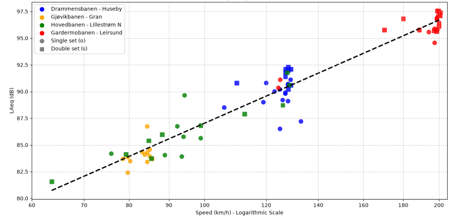
The example supports using a coefficient near 30 for those measurements, but does not establish one coefficient for every train or track. Ursin also reports site-specific estimates of \(29.0\pm4.2\) at Lillestrøm and \(27.3\pm3.2\) at Leirsund. A broad speed range helps distinguish the slope from measurement scatter; a large number of almost identical-speed passages may still give a poorly determined slope. Vehicle and track condition, operating mode and site effects must be considered when interpreting the pooled relationship. If the sites also differ in their typical speeds, the pooled slope can mix a speed effect with site differences; it is not automatically the causal speed response at one unchanged site [223].

12.3.2 Traction Noise

Traction noise is generated by the mechanical and electrical systems of the vehicle: diesel engines, cooling fans, gear boxes, electric motors, compressors, and auxiliary equipment. It dominates at low speeds (below 50–80 km/h) and at standstill. Unlike rolling noise, traction noise levels are nearly independent of speed for a given operating mode.

Key traction noise sources include:

• Diesel engines: a broadband noise source, typically 90–100 dB(A) at 7.5 m from modern high-power diesel locomotives.

• Cooling fans: tonal components at blade-passing frequency and harmonics; can be dominant at idle.

• Electric traction systems: inverter switching noise at frequencies related to the switching frequency (typically 300–3000 Hz); increasingly relevant for EMU fleets.

• Compressors and auxiliary equipment: significant at stations and during dwell.

Modern traction systems (permanent magnet motors, high-switching-frequency inverters, enclosed gear boxes) have substantially reduced traction noise over the past two decades, so that rolling noise is now the dominant source for most modern electric multiple units (EMUs) above 60–80 km/h [158, 68].

The lecture distinguishes low-speed starting noise from steady pass-by noise. Acceleration involves changing traction load, fan demand and auxiliary operation, so a low train speed does not necessarily imply a low sound level. A measurement or prediction should specify the operating state as well as the speed [223].

12.3.3 Stationary Noise

A train at standstill produces no rolling noise, but it may continue to radiate substantial sound from idling engines and auxiliary systems. Sources include heating, ventilation and air-conditioning equipment; converter and transformer cooling fans; compressors and exhaust valves; auxiliary generators; and refrigeration equipment on freight vehicles. Some sources are tonal, while others operate intermittently [223].

Stations, signals, depots and stabling yards therefore require an operating-state assessment. Useful measures include an energy-saving parking mode, shore power where it can replace diesel idling, appropriate stabling locations, and scheduling pre-heating and departures to reduce exposure near dwellings. Any change must retain the functions needed for vehicle safety, readiness and passenger comfort. Stationary noise and traction noise have overlapping equipment sources, but different operating conditions and assessment procedures.

12.3.4 Aerodynamic Noise

At high speeds (\(v > 200\) km/h) aerodynamic noise becomes increasingly important and eventually dominates the total noise level. The main aerodynamic noise sources are:

• Bogies and undercarriage: turbulent flow around the bogie cavity is the largest source on most high-speed trains.

• Pantograph: a significant discrete source; pantograph-related noise can exceed rolling noise at speeds above 280 km/h.

• Inter-car gaps: flow separation and cavity resonances in the gaps between coaches.

• Nose and tail: pressure disturbances propagate as travelling waves along the train length.

Aerodynamic noise grows approximately as \(60\log_{10}(v/v_0)\), i.e. by about 18 dB per doubling of speed, much faster than rolling noise. At 300 km/h, each 10 km/h increase in speed adds approximately 0.9 dB(A). Equivalently, each 25 km/h increase adds approximately 2 dB(A) [158].

12.3.5 Impact Noise

Impact noise arises from discontinuities in the running surface:

• Rail joints and insulated joints: a wheel crossing a gap generates a sharp impulsive force. Welded track (CWR) has largely eliminated this source on main lines, but insulated block joints in signalling systems remain a problem.

• Switches and crossings: the wheel transitions from the running rail onto the crossing frog, creating both a geometric gap (crossing nose) and a change in rail head height. The resulting impact force radiates as a loud impulse, typically 5–10 dB above the rolling noise level for the same train speed.

• Wheel flats: a flat spot on the wheel tread, caused by wheel locking during braking, generates a repetitive impact at a frequency equal to the train speed divided by the wheel circumference. Even a 50 mm flat is clearly audible and generates excessive dynamic forces (see Chapter 10).

Wheel-Flat Geometry and Dynamic Force

A wheel flat repeats approximately once per revolution. For wheel diameter \(D\) and speed \(v\) in m/s, the repetition frequency is

\[ f_{\mathrm{flat}}=\frac{v}{\pi D}. \]

At 100 km/h and \(D=0.92\) m, this is about 9.6 Hz. The short contact-force pulse contains frequencies above this repetition frequency, so a low repetition rate does not imply that the resulting noise is only low-frequency sound.

For an ideal fresh flat of chord length \(l_0\) on a wheel of radius \(R\), simple circular geometry gives, for \(l_0\ll R\),

\[ d\approx\frac{l_0^2}{8R}. \]

Wear changes the shape and edge sharpness. Two flats of the same length can therefore generate different impact loads. A measured worn defect need not follow the chord-depth relation for an ideal fresh flat. The lecture illustrates partial unloading followed by an impact peak and cites a field-test example in which the maximum force occurs around 40 km/h for a roughly 100 mm by 0.9 mm defect. This is a case-specific response, not a general critical speed [223].

Wayside wheel-impact measurement systems assess the force consequence directly, complementing dimensional inspection of the wheel. Acceptance limits must be taken from the applicable maintenance standard and vehicle conditions; a single flat-length value should not be treated as universal. A clearly audible impact also need not imply that a dimensional limit has already been exceeded.

12.3.6 Rail Corrugation

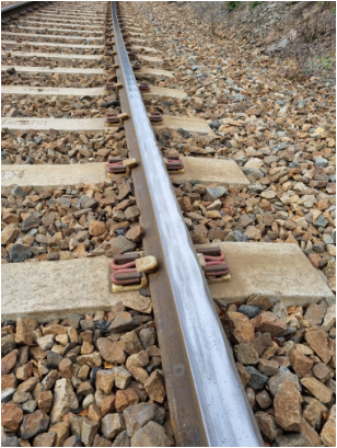
Rail corrugation: short-pitch (20–80 mm) periodic rail roughness generates a strong tonal noise component at the corrugation frequency \(f = v / \lambda_c\); for \(\lambda_c = 30\) mm and \(v = 100\) km/h, \(f \approx 925\) Hz. Because corrugation is periodic, residents often describe the resulting tonal noise as a "singing" or "howling" sound, and the same repeated excitation also raises dynamic wheel–rail forces and accelerates track degradation [105, 106].

The lecture adds a photograph of severe corrugation on the Roa–Hønefoss line, taken by Torbjørn Ursin in 2021. The repeated surface pattern provides a field example of the periodic excitation described above [223].

The repeated rail-surface pattern in Figure 12.7 is the physical counterpart of periodic roughness excitation. Its wavelength must be considered with train speed to relate the surface pattern to an excitation frequency.

Figure 12.7 Rail corrugation on the Roa–Hønefoss line. Photo: Torbjørn Ursin, 2021 [223].

12.3.7 Brake Noise and Curve Squeal

Brake squeal and roughness from tread braking are different mechanisms. Brake squeal is tonal noise caused by friction-induced vibration in the braking system. Cast-iron tread-brake blocks can also roughen the wheel tread, increasing rolling noise even when the train is not braking. Composite brake blocks can keep the tread smoother and reduce this rolling noise. K-blocks have higher friction and require a suitably adapted braking system; they are not a direct replacement for cast-iron blocks. LL-blocks were developed for retrofitting with friction characteristics closer to cast iron, within approved conditions of use. UIC's freight-noise work links K- and LL-blocks to reduced freight rolling noise [114]. See also UIC's comparison of K- and LL-blocks [205].

Brake arrangement	Wheel-tread condition and noise implication	Compatibility consideration
Cast-iron tread blocks	Can roughen the tread and raise rolling noise away from the braking event.	Existing braking performance and maintenance requirements still apply.
Composite K-blocks	Can maintain a smoother tread.	Higher friction generally requires an adapted braking system.
Composite LL-blocks	Can maintain a smoother tread with friction characteristics closer to cast iron.	Retrofitting is subject to approved conditions of use.
Disc brakes	Avoid direct brake-block roughening of the running tread.	Vehicle design and braking-system compatibility govern implementation.

Table 12.2 Brake arrangements, tread condition and noise.

The acoustic benefit of changing blocks depends on both surfaces: a smooth wheel still runs noisily on a rough rail. Climate, braking performance and authorisation also matter, so a block material should not be selected from noise reduction alone [223].

Two Wheel–Rail Contact Situations

Curve squeal is strong tonal noise caused by friction-induced wheel–rail vibration, often associated with lateral sliding at the tread contact in tight curves. Falling friction and coupling between vibration modes can both produce instability; stick-slip is not the only explanation. Wheel modes in the range 500–4000 Hz can be involved, but neither that range nor a radius of 300 m is a universal boundary. Squeal occurrence and level depend on wheel and rail profiles, friction, vehicle dynamics and the measurement position [158]. See Ding et al.’s comparison of squeal mechanisms [206]. Mitigation can include approved top-of-rail friction modifiers or wheel damping. Gauge-face lubrication addresses flange contact and must be controlled so that lubricant does not contaminate the running surface and reduce braking adhesion.

Figure 12.8 separates flange contact at the high rail from sliding at the tread contact. The exaggerated angle of attack clarifies the geometry; it should not be read as a measured operating angle or as proof that both contacts have the same squeal mechanism.

Figure 12.8 Flange contact and tread sliding in a curve. The angle of attack is exaggerated. From Torbjørn Ursin’s lecture [223].

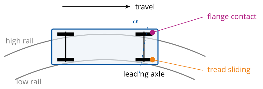
The lecture distinguishes flange contact at the high rail from lateral sliding at the tread contact. Both can generate friction-related sound, but flange noise and tread-contact curve squeal should not be assumed to have the same instability mechanism. Worn or mismatched profiles can worsen steering and contact conditions; curve radius, angle of attack and the rolling-radius difference available to the wheelset also matter. Profile measurement is therefore part of diagnosis, rather than proof that wear is always the cause [223].

Gauge-face lubrication addresses flange contact. Top-of-rail friction management addresses the tread-contact condition and must use an approved product and application rate. Wheel or rail reprofiling can restore the intended contact geometry. The measure should follow the observed contact situation, with braking and traction adhesion retained.

In practice, curve-squeal mitigation is usually a trackside maintenance and friction-control problem. The contact diagram above distinguishes the locations that require different friction-control measures.

12.4 Ground-Borne Vibration

Ground-borne vibration is treated separately from airborne noise because the transmission path, frequency range, and mitigation measures are different. The following subsections trace the vibration from the wheel–rail contact into the ground and nearby buildings. Simultaneous noise and vibration can affect perception of the combined exposure, so an assessment should consider both routes instead of interpreting a vibration measurement without its acoustic context [223].

12.4.1 Generation Mechanism

Ground-borne vibration is generated by the dynamic wheel–rail forces described in Chapter 10. The oscillating contact forces propagate downward through the rail and fastening system into the sleepers and ballast (or slab), and from there into the ground as elastic waves. The dominant frequency range is approximately 4–200 Hz [158].

The main vibration excitation mechanisms are:

• Quasi-static deflection: the ground deflects under the passing train weight, creating a slowly moving elastic bowl that is felt as a low-frequency (\(< 10\) Hz) disturbance in the near field.

• Dynamic roughness excitation: wheel and rail roughness excite dynamic forces at frequencies from about 20 to 2000 Hz. Ground-borne vibration in the 20–200 Hz range from this source propagates as body waves (P and S waves) and surface Rayleigh waves.

• Parametric excitation: the periodic variation in track stiffness between mid-sleeper-bay and directly above a sleeper generates an excitation at the sleeper-passing frequency \(f_{sp} = v / d_s\) (where \(d_s\) is the sleeper spacing, typically 0.6 m).

At 100 km/h and a sleeper spacing of 0.6 m, the sleeper-passing frequency is about \(27.8/0.6=46\) Hz. This identifies one excitation frequency; it does not predict the received vibration without the track, ground and building transfer responses.

12.4.2 Wave Propagation in the Ground

The lecture first distinguishes body waves from surface waves. In a P-wave, particle motion is parallel to propagation; in an S-wave it is transverse. Rayleigh waves involve elliptical particle motion near the surface. Love waves involve horizontally polarised shear motion and depend on a suitable layered ground structure. These descriptions concern particle motion, not the direction in which a train travels [223].

Compare particle motion with propagation direction in Figure 12.9. P- and S-waves are body waves, whereas Rayleigh and Love waves are associated with the surface; the animations illustrate motion patterns rather than the direction of train travel.

(a) P-wave

(b) S-wave

(c) Rayleigh wave

(d) Love wave

Figure 12.9 Body waves (P and S) and surface waves (Rayleigh and Love). Animations: L. Braile [237], via Ursin [223].

For a homogeneous, isotropic, linear-elastic material, the body-wave velocities depend on the elastic moduli and density [239]:

• P-waves are compressional body waves with velocity \(c_P = \sqrt{(K + 4G/3)/\rho}\).

• S-waves are shear body waves with velocity \(c_S = \sqrt{G/\rho}\).

• Rayleigh waves are surface waves with motion concentrated near the ground surface. Their contribution to railway vibration depends on the excitation, ground conditions, frequency and distance [113].

Figure 12.10 Idealised geometric spreading of body and surface waves, with r₀ = 5 m. Material damping and layering are excluded.

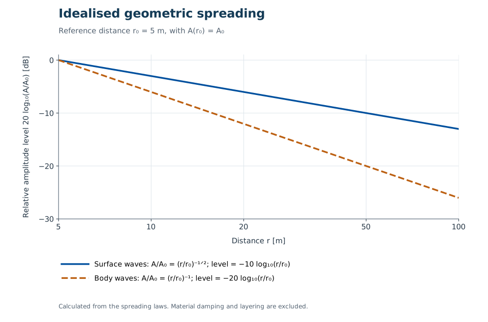
Figure 12.10 compares idealised amplitude decay from cylindrical surface-wave spreading, proportional to \(r^{-1/2}\), and spherical body-wave spreading, proportional to \(r^{-1}\). The 5 m reference distance normalises the plotted levels; it is not a threshold for Rayleigh-wave dominance. Material damping, layering, frequency and source geometry affect propagation at a real railway site [113].

Here \(K\) is the bulk modulus, \(G\) is the shear modulus, and \(\rho\) is the mass density of the ground material.

The relative importance of these wave types changes with soil layering, distance, and frequency. A useful practical distinction is that soft ground is often associated with noticeable vibration, while hard ground can transmit vibration efficiently into buildings where it is re-radiated as structural noise.

12.4.3 Building Response and Re-radiated Noise

When ground vibration reaches a building foundation, it is transmitted through the structural system (columns, slabs, walls) to the floors and ceilings. The floor and ceiling vibration radiates as low-frequency airborne sound, known as structure-borne noise or re-radiated noise. This manifests as a low-frequency "rumble" inside the building that is difficult to treat with conventional sound insulation, because the noise arrives via the structure rather than through the facade.

The frequency range of re-radiated noise is typically 16–250 Hz. Assessment uses both vibration metrics (velocity level \(L_v\) in dB re \(10^{-9}\,\mathrm{m\,s^{-1}}\) or acceleration level \(L_a\) in dB re \(10^{-6}\,\mathrm{m\,s^{-2}}\)) and acoustic metrics (sound pressure level in dB(A) or dB(C) for very low frequencies) [158].

12.4.4 Comparing Frequency Ranges

The overlapping bands in Figure 12.11 help distinguish felt vibration, re-radiated sound and airborne noise without imposing sharp physical boundaries. The illustrated frequency ranges are descriptive, not regulatory acceptance limits.

Figure 12.11 Indicative frequency ranges for noise, vibration and hearing. From Torbjørn Ursin’s lecture [223].

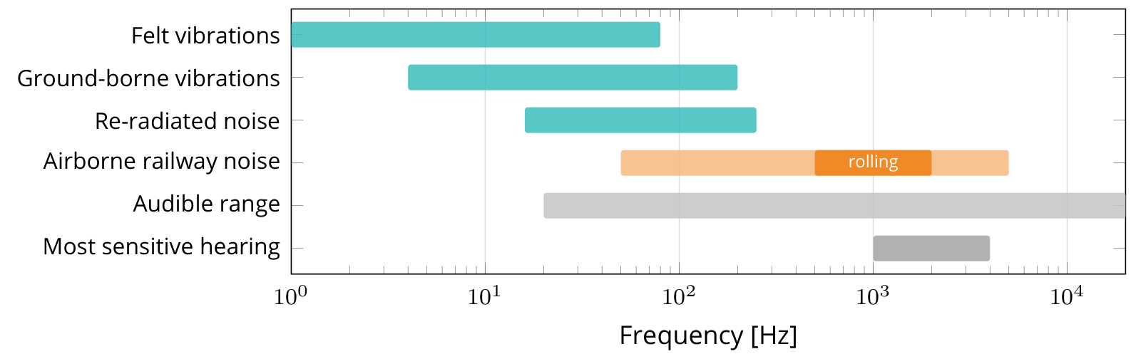
Felt vibration, ground-borne vibration, re-radiated indoor noise and directly airborne railway sound occupy overlapping frequency ranges. These descriptions should be distinguished without treating their frequency boundaries as assessment limits. A vibration can be below the nominal audible range yet remain perceptible through the body; the same excitation can also produce audible sound when it excites a building element. Measurements should retain sufficient spectral information to distinguish these effects [223].

12.5 Noise Assessment and Requirements

Noise assessment requires both a physical quantity and a regulatory context. This section therefore introduces the acoustic indicators before linking them to Norwegian limit values and mitigation decisions.

12.5.1 Interpreting a Change in Decibels

Decibel levels express a logarithmic ratio. If two statistically independent sound contributions have equal mean-square pressure at a receiver, combining them raises the level by approximately 3 dB. Doubling the number of otherwise identical train events likewise raises the equivalent level over a fixed period by about 3 dB. It does not double the maximum level of each event [223].

Level change	Indicative perception in the lecture
1–2 dB	Often difficult to notice.
3–4 dB	Noticeable under suitable comparison conditions.
5–7 dB	A considerable change.
8–10 dB	Often described approximately as halving or doubling loudness.

Table 12.3 Indicative perception of changes in sound level.

These are listening rules of thumb, not guaranteed responses. Frequency, duration, background noise and the listener influence perception. A 10 dB increase represents ten times the acoustic energy, although it is often perceived as roughly twice as loud. A 12 dB increase corresponds to an energy ratio \(10^{12/10}\approx16\). The same ratio applies to traffic counts only if event emissions, timing and other assessment conditions remain unchanged.

The earlier rolling-noise example, 120 to 160 km/h, gives a 3.7 dB increase. The table makes the practical meaning of that change clearer, while the separate event count and speed relations explain why a traffic forecast needs both quantities.

12.5.2 Acoustic Quantities

The fundamental quantity for noise assessment is the A-weighted sound pressure level \(L_A\), calculated as \(L_A = 10 \log_{10}(p_A^2/p_\text{ref}^2)\) in dB(A), where \(p_A\) is the A-weighted root-mean-square pressure and \(p_\text{ref} = 20\,\mu\mathrm{Pa}\) is the reference sound pressure. The A-weighting filter approximates the frequency sensitivity of the human ear at moderate sound levels, attenuating very low (\(< 100\) Hz) and very high (\(> 8000\) Hz) frequencies.

For railway noise assessment, the most important acoustic indicators are listed below. This table defines what each indicator measures; the Norwegian planning and action values are summarised separately in Table 12.7.

Indicator	Use in railway-noise assessment
\(L_{Aeq,T}\)	Equivalent continuous A-weighted level over a time period \(T\).
\(L_{Amax}\)	Maximum A-weighted pass-by level; used in sleep-disturbance assessment. For Norwegian railway planning, the statistical form \(L_{5AF}\) is used.
\(L_{den}\)	Day–evening–night equivalent level for mapping and planning.
\(L_{night}\)	Nighttime equivalent level, 23:00–07:00; linked to sleep disturbance.

Table 12.4 Indicators used in railway-noise assessment.

The notation \(L_{5AF}\) is compact but important. The subscript 5 means the A-weighted maximum level exceeded by 5% of the relevant noise events, such as individual train pass-bys. The letter A denotes A-weighting, and F denotes the "Fast" 125 ms time weighting. It is therefore a statistical maximum level, not necessarily the single loudest train event in the period [123].

The day–evening–night indicator is an energy average with penalties added to evening and nighttime exposure:

\[ \begin{aligned} L_{den} &= 10\log_{10}\!\Biggl[\frac{1}{24}\!\Bigl( 12 \cdot 10^{L_d/10} + 4 \cdot 10^{(L_e+5)/10}\\ &\qquad\qquad {}+ 8 \cdot 10^{(L_n+10)/10} \Bigr)\Biggr]. \end{aligned} \]

(12.1)

Here \(L_d\), \(L_e\) and \(L_n\) are the daytime (07:00–19:00), evening (19:00–23:00) and nighttime (23:00–07:00) levels. The evening and nighttime penalties are 5 dB and 10 dB respectively.

Worked example.

Suppose \(L_d = 60\) dB(A), \(L_e = 55\) dB(A) and \(L_n = 50\) dB(A). After the evening and night penalties, all three energy terms become equivalent to 60 dB(A):

\[ L_{den} = 10\log_{10}\!\left[ \frac{12\cdot10^{6} + 4\cdot10^{6} + 8\cdot10^{6}}{24} \right] = 60\,\text{dB(A)}. \]

The example shows why nighttime railway noise is important even when the measured nighttime equivalent level is lower than the daytime level.

12.5.3 Determining Noise Exposure

Large-area exposure assessments normally combine a source model with a propagation model. Long-term measurements at every dwelling are costly and may not represent the intended traffic scenario. Calculation allows existing, future and mitigated cases to be compared on consistent assumptions; measurements remain important for source characterisation, checks and investigation of individual events [223].

Stage	Information and decisions
Input	Train type, number, speed, length and operating state; track type and condition; terrain, ground, meteorology, buildings and receiver height.
Method	A compatible emission model and propagation method, implemented in an appropriate calculation tool.
Output	Noise maps and zones, levels at building facades and the required indicators such as equivalent level, \(L_{den}\) and event maxima.
Check	Confirm that traffic data, emission data, surface condition, receiver positions and the calculation method match the assessment purpose.

Table 12.5 Inputs, method and checks in a railway-noise calculation.

The lecture gives CadnaA, SoundPLAN and Norstøy as examples of tools. A software name alone does not identify the calculation method or validate its inputs. Source data are often decisive: an inaccurate fleet mix, speed, operating mode or roughness assumption can dominate a carefully modelled propagation path.

Measurement standards also have distinct purposes. NS 8177 concerns noise received from railway traffic, while EN ISO 3095 addresses railway-vehicle emission measurements under specified conditions, including the test track. A vehicle result from a reference-track test cannot be substituted directly for the exposure at a particular dwelling.

12.5.4 Railway-Noise Calculation Methods

Ursin compares three method families used for railway-noise assessment. Their source descriptions, frequency bands and propagation corrections differ, so their input data and results are not interchangeable [223].

Feature	Nord96	Nord2000	CNOSSOS-EU
Basis	Nordic railway-noise prediction method published in 1996.	Nordic development combining source descriptions with detailed propagation modelling.	Harmonised method for assessment under the Environmental Noise Directive.
Frequency description	Octave bands, 63 Hz–4 kHz [234].	One-third-octave bands, 25 Hz–10 kHz [233].	Octave-band propagation, 63 Hz–8 kHz; railway sources are calculated in one-third-octave bands before energy summation [235, 73].
Source representation	Measured emission for train types with speed dependence and corrections.	Band sound powers for vehicle categories with operating and track corrections.	Separate train and track source mechanisms assembled into category emissions.
Propagation treatment	Engineering corrections for distance, ground and screening.	Terrain, ground impedance, screening and meteorological profiles.	Defined propagation procedures for homogeneous and favourable conditions.
Main assessment context	Established planning applications.	Detailed planning and environmental studies.	Strategic mapping and reporting under the European framework.

Table 12.6 Railway-noise prediction methods compared in the lecture.

M-2061 Section 9.5 lists Nord2000, the Nordic 1996 method and CNOSSOS as accepted methods for railway-noise calculation. It requires the choice of method and the uncertainty to be explained [224]. Record the method, version and assumptions for each assessment. A more detailed model does not automatically give a better answer if its source and site data are weak. Check current national guidance before selecting a method for a new project.

12.5.5 Norwegian Regulatory Framework

Norwegian railway-noise assessment should keep three regulatory contexts separate. Table 12.7 summarises the main values used for planning, zoning and existing-activity follow-up.

Context	Indicator	Railway value	Use in assessment
T-1442 planning value	\(L_{den}\)	\(\leq 58\) dB	Outside windows in rooms with noise-sensitive use and on the quiet part of outdoor amenity areas.
T-1442 night maximum	\(L_{5AF}\)	\(\leq 75\) dB	Outside bedroom windows for night periods with more than ten railway events.
T-1442 yellow zone	\(L_{den}\) or \(L_{5AF}\)	\(>58\) dB or \(>75\) dB	Assessment zone where noise-sensitive development requires careful planning and mitigation.
T-1442 red zone	\(L_{den}\) or \(L_{5AF}\)	\(>68\) dB or \(>90\) dB	Zone generally unsuitable for new noise-sensitive use unless justified in priority development areas.
Pollution Regulations Chapter 5	\(L_{pAeq,24h}\) indoors	\(>42\) dB	Action threshold for existing activities and existing buildings.

Table 12.7 Key Norwegian railway-noise planning and action indicators.

T-1442 values are planning-guideline values. Binding project requirements are set through plans, permits, building regulations, and project-specific conditions.

The table should be read together with the regulatory context:

• T-1442/2021: the Norwegian government's noise guidelines for land-use planning and new noisy infrastructure. For railway noise, the main planning indicator is \(L_{den}\), with a separate nighttime maximum-level indicator \(L_{5AF}\) outside bedrooms when there are more than ten events per night [123].

• Pollution Control Regulations. Chapter 5 of Forurensningsforskriften governs mapping, action plans, and thresholds for existing activities. Its central action threshold is an indoor \(L_{pAeq,24h}\) value, not the outdoor railway planning value in T-1442 [131].

• EU Directive 2002/49/EC: requires strategic noise mapping and action plans for major railways and agglomerations [95, 73].

The practical review point is that \(L_{night}\), \(L_{5AF}\), and indoor \(L_{pAeq,24h}\) answer different questions. They should not be substituted for one another without checking the applicable regulation or project condition.

12.5.6 Requirements and Measurement Standards

Regulations establish duties and requirements, while standards specify quantities, test arrangements and assessment procedures. They should be selected according to the source and receiver being studied. The lecture maps the following principal documents [223].

Assessment task	Relevant framework or standard family
Strategic environmental-noise mapping	Directive 2002/49/EC and the common methods in Directive (EU) 2015/996, as amended.
Railway-vehicle noise requirements	TSI Noise, Regulation (EU) 1304/2014, as amended.
Historical noise-related charging scheme	The scheme under Regulation (EU) 2015/429 ended in 2021; the act was repealed by Regulation (EU) 2024/327 [231]. It should not be cited as a current charging requirement.
Stationary, starting and pass-by vehicle emissions	EN ISO 3095.
Noise inside railway vehicles	ISO 3381.
Wheel and rail roughness	EN 15610.
Track decay rates	EN 15461.
Railway noise barriers	EN 16272 series.
Description and measurement of environmental noise	ISO 1996 series.
Ground-borne vibration and resulting building noise	ISO 14837-1.
Norwegian land-use planning and existing-source exposure	T-1442 with M-2061; Chapter 5 of Forurensningsforskriften.
Building acoustic and vibration performance	TEK17 and the applicable NS 8175 and NS 8176 assessment provisions.
Received noise from railway traffic	NS 8177.
Infrastructure design and maintenance	Bane NOR technical regulations.

Table 12.8 Principal regulatory and measurement frameworks.

A standard is not automatically a universal legal limit. Its edition, scope and route of application through regulations, a plan, permit or contract must be established. TEK17 Section 13-6 requires satisfactory sound and vibration conditions; its guidance identifies NS 8176:2017 for vibration assessment, while Class C in NS 8175:2012 provides a route to satisfying the building-sound requirement [225]. This does not turn every listed standard or every Class C value into one universal railway limit. European railway requirements likewise need to be read with their scope, amendments and implementation in Norway [232].

12.5.7 Vibration Measurement

Ground-borne vibration is quantified by the vibration velocity level \(L_v\) (in dB re \(10^{-9}\,\mathrm{m\,s^{-1}}\)) measured at octave or one-third octave bands. ISO 14837-1:2005 [113] gives general guidance on ground-borne vibration and resulting noise in buildings from railway operation. It covers source, propagation and receiver effects; it does not set a universal vibration limit or cover construction vibration. The Norwegian standard NS 8176 specifies vibration classes for dwellings using the statistical maximum weighted velocity \(v_{w,95}\):

NS 8176 class	Statistical maximum weighted velocity \(v_{w,95}\)
A	\(\leq0.10\) mm/s
B	\(\leq0.15\) mm/s
C	\(\leq0.30\) mm/s
D	\(\leq0.60\) mm/s

Table 12.9 Vibration classes for dwellings in NS 8176.

Classes A and B represent stricter comfort levels that may be used where a high vibration standard is required, while Class D is a less demanding class for cases where Class C is not practical. Class C is commonly used as a planning target for new land-based transport infrastructure near dwellings, but the exact requirement must be checked for the specific project [113, 156]. The class values are reproduced in Bane NOR’s vibration guidance [207]; NS 8176:2017 is the Norwegian edition used here.

Vibration velocity levels in frequency bands and the weighted statistical value \(v_{w,95}\) serve different purposes and should not be interchanged. The absence of one general remedial threshold for existing buildings does not establish that all existing vibration is acceptable; the applicable planning, building, environmental and project requirements still need to be identified.

12.6 Mitigation Measures

Mitigation of railway noise and vibration can be applied at three levels: at the source (vehicle and track), along the propagation path, and at the receiver (building facade). Source-based measures are generally most cost-effective.

The lecture organises these measures as avoid, reduce and mitigate, following Bane NOR’s Unngå, begrense, avbøte approach. First avoid unnecessary excitation or exposure through planning. Then reduce roughness, dynamic force, radiation or propagation. Finally mitigate the remaining exposure, for example through local facade measures. This is a priority order, not an exclusive source–path–receiver classification: Bane NOR’s project guidance also includes near-source barriers among reduction measures. See the lecture [223].

12.6.1 Avoiding Noisy Events

At the infrastructure source, continuously welded rail removes ordinary joints and movable-point crossings can remove the gap encountered at a fixed crossing nose. Profile maintenance and suitable friction management can prevent or reduce recurring squeal. At the vehicle source, brake maintenance and wheel-condition monitoring can reduce the likelihood of wheel-flat impacts. These measures can also reduce damaging dynamic loads [223].

Operational and land-use planning can place stabling, shunting and terminal activity away from sensitive receivers, reduce unnecessary idling and schedule noisy preparation work appropriately. Layout or operational changes may remove the routine need for some warning events, but required safety signals and horn use must be retained [230]. Avoiding exposure is a planning decision, not permission to suppress a required warning.

12.6.2 Rail Grinding for Rolling Noise

Rail grinding (described in Chapter 17) removes surface material to restore a smooth rail profile, reducing both rail corrugation and roughness. In Bane NOR practice, rail grinding is not specified as one universal calendar interval: the rail-maintenance rules treat grinding, milling, or planing as condition-triggered actions to be carried out no later than the permitted wave-depth limit for rail corrugation and waves is reached. A separate gross-tonnage rule applies to weld finishing: in trafficked track, final grinding must be performed as soon as possible and before more than 30 000 gross tonnes have passed over the weld [13, 11]. The noise mechanism is the reduction of surface roughness and corrugation that excite wheel and rail vibration. Rail grinding is therefore one of the most cost-effective rolling-noise mitigation measures available to the infrastructure manager [105, 130].

12.6.3 Brakes, Low-Noise Wheels and Damped Wheels

Wheel vibration accounts for up to 30% of total rolling noise energy on some vehicles. Mitigation measures applied to the wheel include:

• Wheel dampers: designs include tuned absorbers, ring dampers and constrained-layer damping treatments. They act on radiating wheel modes; reductions of 3–8 dB in wheel-radiated noise are system-specific and do not necessarily give the same reduction in total train noise.

• Optimised wheel profiles: suitable profiles and reprofiling maintain the intended contact geometry and steering behaviour. Roughness and squeal must still be assessed separately; reducing equivalent conicity alone is not a general acoustic design rule.

• Composite brake blocks: K-blocks that produce a smooth tread surface, reducing tread roughness and hence rolling noise by 8–12 dB compared with cast-iron block-braked vehicles [158].

In Bane NOR's public technical-regulation material, low-noise wheel design is handled indirectly rather than through one prescribed damper geometry. The rail-maintenance rules control the wheel–rail interface by evaluating track equivalent conicity against reference wheel profiles such as S1002 and GV 1/40, with speed-dependent limit values. The Network Statement also requires frequency-based noise-emission data when new rolling stock is introduced on the national railway network, or when modifications to existing rolling stock change the nature of the noise emission. These requirements support acoustic acceptance and compatibility checks, but they should not be read as a standard drawing of a particular damped-wheel construction [13, 37].

The lecture reports a German example of about 13 dB reduction from a combination of cast-iron-to-LL-block conversion and acoustic grinding. This is a combined treatment result, not a reduction attributable to either measure independently. It illustrates the benefit of improving both wheel and rail condition [223].

TSI Noise addresses vehicle emission requirements, including stationary, starting and pass-by tests, and includes provisions for quieter routes and freight wagons [226]. ERA defines a quieter route as at least 20 km long with an average of more than 12 freight trains per night under the specified counting conditions. The corresponding provisions apply from December 2024, with temporary non-application on the Finnish and Swedish networks until 31 December 2032 [227]. These provisions restrict operation of wagons outside the specified noise-performance conditions; they should be applied using the route, wagon and exemption rules rather than treated as an unrestricted ban on a brake material everywhere.

12.6.4 Rail Dampers

Rail dampers are absorbers attached to the rail web and foot to increase attenuation of rail vibration. Increasing track decay rate shortens the radiating rail length and can reduce the rail contribution to rolling noise. Their effectiveness depends on the untreated track dynamics and on how much of the total noise originates in the rail [223].

Figure 12.12 Freight-train TEL spectra at 101 km/h in Tjörnarp, with and without rail dampers. Replotted from Nielsen et al. [242].

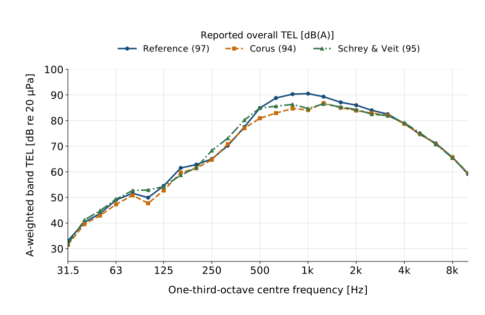
The original QCITY report [242] documents the Swedish field test at Tjörnarp in September 2008. For freight passage 1 at 101 km/h, it reports overall TEL values of 97 dB(A) for the reference section, 94 dB(A) with Corus dampers and 95 dB(A) with Schrey & Veit dampers. Much of the difference is in the 500–1600 Hz bands. Figure 12.12 uses the published band values without further weighting or roughness correction. These are results for this comparison and these test conditions, not guaranteed reductions for every installation. Measurements were taken 7.5 m from track centre and 1.2 m above the rail. The source spectra are already corrected to the reference-section rail roughness.

A 3 dB reduction is meaningful in energy terms, but the engineering decision also depends on receiver exposure, life-cycle cost, maintenance access and alternative measures. If wheel radiation dominates, reducing only the rail contribution has a limited effect. Dampers may be particularly relevant where the rail has a low decay rate, including some tracks with soft pads.

12.6.5 Resilient Components

Resilient track components reduce noise and vibration by changing the vertical stiffness and damping between the rail, sleeper, ballast, slab and tunnel invert. The component must be selected together with the rest of the support system: making one layer softer can reduce vibration transmission, but excessive total deflection can create geometry, stability or resonance problems.

Figure 12.13 locates resilient interfaces at different levels of the track support. Read the positions as alternatives to assess within the complete support system, not as instructions to combine every layer shown.

Figure 12.13 Possible resilient-layer locations, not a combined track arrangement. From Torbjørn Ursin’s lecture [223].

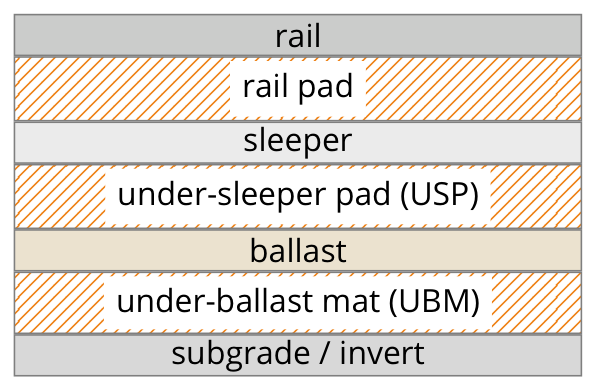
The lecture diagram identifies possible layer locations, not a recommendation to install all layers together. In Bane NOR track, under-sleeper pads and under-ballast mats must not be combined, as explained below.

Resilient layers may be placed at different interfaces, but should not all be installed together without a system-level assessment. The total support stiffness, dynamic amplification and resulting deflection must be evaluated for the selected system.

Rail pads and elastic fastenings. Standard elastic rail fastenings (e.g. Pandrol, Vossloh) use a rail pad to control rail-seat stiffness, peak contact pressure and electrical insulation, as shown in the resilient-layer diagram above. For noise and vibration mitigation, softer rail pads or under-rail pads can attenuate force and vibration transmission from rail to sleeper in the target frequency range. They do not automatically reduce rolling noise: reducing pad stiffness can lower the track decay rate and increase rail vibration and sound radiation. Pad stiffness and damping must therefore be selected from a system-level assessment. As one system-specific example, the FTA manual [208], describes direct-fixation fasteners of about 30,000 lb/in (5.3 kN/mm) that may reduce ground-borne vibration by 5–10 dB above 30–40 Hz. This is not a guaranteed airborne-noise reduction or a specification for ordinary rail pads [158, 68].

Frequency-Dependent Rail-Pad Design: LowNoisePad

The LowNoisePad example addresses the conflict between flexible support and rail sound radiation. The aim is to retain suitable low-frequency track behaviour while providing a dynamic response that increases rail-vibration decay in acoustically important bands. It therefore treats pad performance as frequency-dependent rather than describing a pad by one stiffness value [223].

The UIC LowNoisePad final report describes test reductions of approximately 3–5 dB relative to soft standard pads and 1–2 dB relative to stiff pads, depending on the participating test conditions [228]. These are measured comparison results, not a guaranteed reduction across an entire network. Ursin describes the collaboration of 12 infrastructure managers, including Bane NOR, and reports a Norwegian test installation with deployment on Trønderbanen planned for 2027. The Norwegian deployment statement is lecture evidence from October 2026; the plan is not evidence of a completed installation [223].

Replacing pads during planned track renewal may allow acoustic improvement with little additional installation work. Whole-life performance still requires checks of durability, mechanical and electrical functions, track deflection and maintenance compatibility. A small added component cost does not by itself establish zero project or life-cycle cost.

Resilience Beneath Sleepers and Ballast

Under-sleeper pads (USPs). Under-sleeper pads are resilient elastomeric layers bonded to the underside of concrete sleepers, as shown in the resilient-layer diagram above. Bane NOR's technical regulations list concrete sleepers supplied with under-sleeper pads and specify their static stiffness classes [49, 47]. USPs act locally at each sleeper–ballast contact. They reduce the dynamic stiffness of the ballast–sleeper interface, reduce impact forces at joints and crossings, and can reduce ground-borne vibration above the sleeper–ballast resonance. They also improve ballast particle behaviour by increasing contact area and reducing local crushing.

Under-ballast mats (UBMs). Under-ballast mats are continuous resilient sheets placed beneath the entire ballast layer, normally on hard subgrade, a tunnel invert, bridge deck or prepared formation. Unlike USPs, which work at discrete sleeper locations, a UBM isolates the ballast bed as a whole. This can improve ground-borne vibration isolation while retaining conventional sleepers and tampable ballast. Very soft mats may reduce track stability and settlement resistance, so stiffness, ballast depth, drainage and maintenance access must be checked together. Bane NOR's technical regulations prohibit combining UBMs with USPs (TRV:07945), or with XPS frost-protection boards (TRV:07946). These restrictions concern the specified systems, rather than every possible frost-protection material [179]. Combined elastic layers require particular attention to resonance and total deflection [10, 158, 130].

Floating Slab Track

Floating slab track (FST). In slab track, tunnels, and other locations without conventional sleeper–ballast contact, resilience is normally provided by under-slab mats, booted sleepers or blocks, or floating slabs [68, 130]. Floating slab track can provide substantial vibration isolation in tunnels and urban environments. The concrete slab rests on springs or elastomeric mounts. The FTA manual [208], reports installed systems with vertical resonance frequencies ranging from 5–10 Hz to 14–17 Hz. Performance must be assessed against the source spectrum and the coupled vehicle, track and ground response. An ideal undamped single-degree-of-freedom isolator tends toward 12 dB additional isolation per octave well above resonance; this asymptote is not a guaranteed insertion loss for a real track. The key principle is that the rails and fasteners are carried by a massive track slab that is dynamically decoupled from the tunnel invert by resilient isolators.

Floating slabs add substantial construction and maintenance costs. Their use should be justified by the required vibration performance and a comparison with other measures; a universal cost multiplier is not reliable across projects [158, 109].

12.6.6 Embedded and Slab Track

Embedded rail systems (see Chapter 2) encase the rail in a continuous elastomeric boot or cast elastomer layer. The elastomeric material provides:

• Vibration isolation when the complete support system is designed for the relevant excitation range. Low natural frequencies such as 5–12 Hz relate to selected isolation systems and should not be assumed for every embedded rail.

• Reduced exposed rail radiation and added damping, with the net rolling-noise benefit depending on the complete track and vehicle system.

• Continuous rail support that can replace discrete rail fasteners, while introducing its own inspection and maintenance needs for the embedding material and interfaces.

Embedded rail is standard in urban tramway and light rail applications and is increasingly used for heavy urban rail [68].

12.6.7 Noise Barriers

Noise barriers are a well-established propagation-path measure. They intercept the direct sound path from the track to receivers and reduce noise by diffraction around the barrier top edge. For an idealised point source and a thin, sufficiently long barrier that blocks the direct sound path, the Kurze–Anderson approximation estimates the single-frequency shielding loss. Using \(IL\) for this ideal free-field estimate, for \(N > 0\):

The expression and the Fresnel-number convention below are also given in Buba et al., DAGA 2024, Equations (1)–(2) [209].

\[ \begin{aligned} IL &\approx 5 + 20 \log_{10}\!\left(\frac{\sqrt{2\pi N}}{\tanh\!\left(\sqrt{2\pi N}\right)}\right),\\ N &= \frac{2\delta}{\lambda}. \end{aligned} \]

(12.2)

At the grazing limit \(N \to 0^+\), this approximation tends to 5 dB. It excludes transmission through the barrier, diffraction around its ends, and ground or reflection effects; a distributed railway source requires contributions from its individual source positions to be combined.

Here \(\delta\) is the path length difference (detour over the barrier top) and \(\lambda\) is the wavelength at frequency \(f\). The Fresnel number \(N = 2\delta/\lambda\) determines the ideal single-frequency performance: the higher \(N\), the greater the insertion loss. In real railway projects, broadband \(L_{den}\) reduction is usually lower because of source height, ground effects, reflections, leakage, receiver height, and the train noise spectrum. Figure 12.14 gives the geometry used to define the wheel–rail noise source, the blocked line of sight, and the diffracted path over the barrier top edge.

Figure 12.14 A noise barrier interrupts the direct sound path; sound diffracts over its top edge.

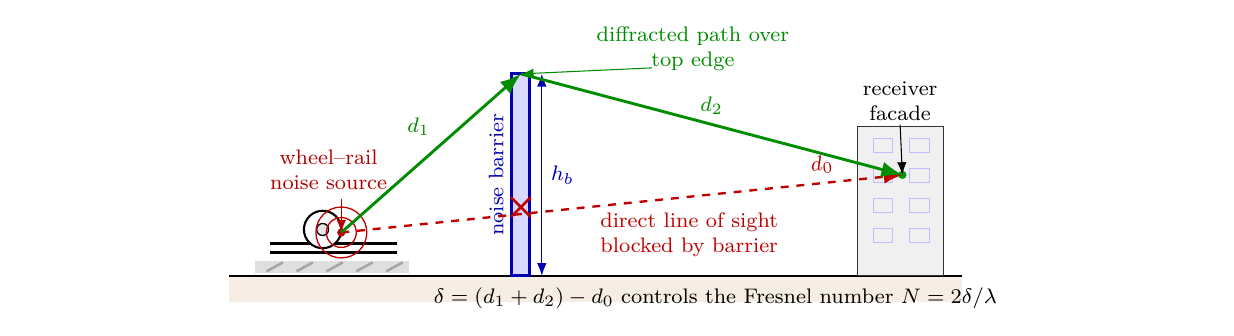
Worked example.

Using Figure 12.14, assume that the barrier blocks the direct line of sight between the wheel–rail source and a receiver. Let the distance from the source to the barrier top be \(d_1 = 3.0\) m, the distance from the barrier top to the receiver be \(d_2 = 6.2\) m, and the unobstructed direct distance be \(d_0 = 9.1\) m. The path length difference is therefore

\[ \delta = (d_1+d_2)-d_0 = (3.0+6.2-9.1)\,\mathrm{m} = 0.10\,\text{m}. \]

For the wavelength calculation, \(c\) is the speed of sound in air and \(f\) is the frequency. At the 500 Hz octave-band centre, using \(c = 340\) m/s,

\[ \begin{aligned} \lambda &= \frac{c}{f} = \frac{340\,\mathrm{m/s}}{500\,\mathrm{s^{-1}}} = 0.68\,\text{m},\\ N &= \frac{2\delta}{\lambda} = \frac{2(0.10\,\mathrm{m})}{0.68\,\mathrm{m}} = 0.29 . \end{aligned} \]

Substituting \(N = 0.29\) in Equation 12.2 gives

\[ \begin{aligned} IL &\approx 5 + 20\log_{10}\!\left( \frac{\sqrt{2\pi(0.29)}}{\tanh\!\left(\sqrt{2\pi(0.29)}\right)}\right)\\ &\approx 8.8\,\text{dB}. \end{aligned} \]

This value should be read as an ideal single-frequency screening estimate. The achievable broadband reduction for a real railway barrier will usually be lower after source height, leakage, reflections, ground conditions, and the train noise spectrum are included. The same geometry gives a larger ideal insertion loss at higher frequencies because the wavelength is shorter.

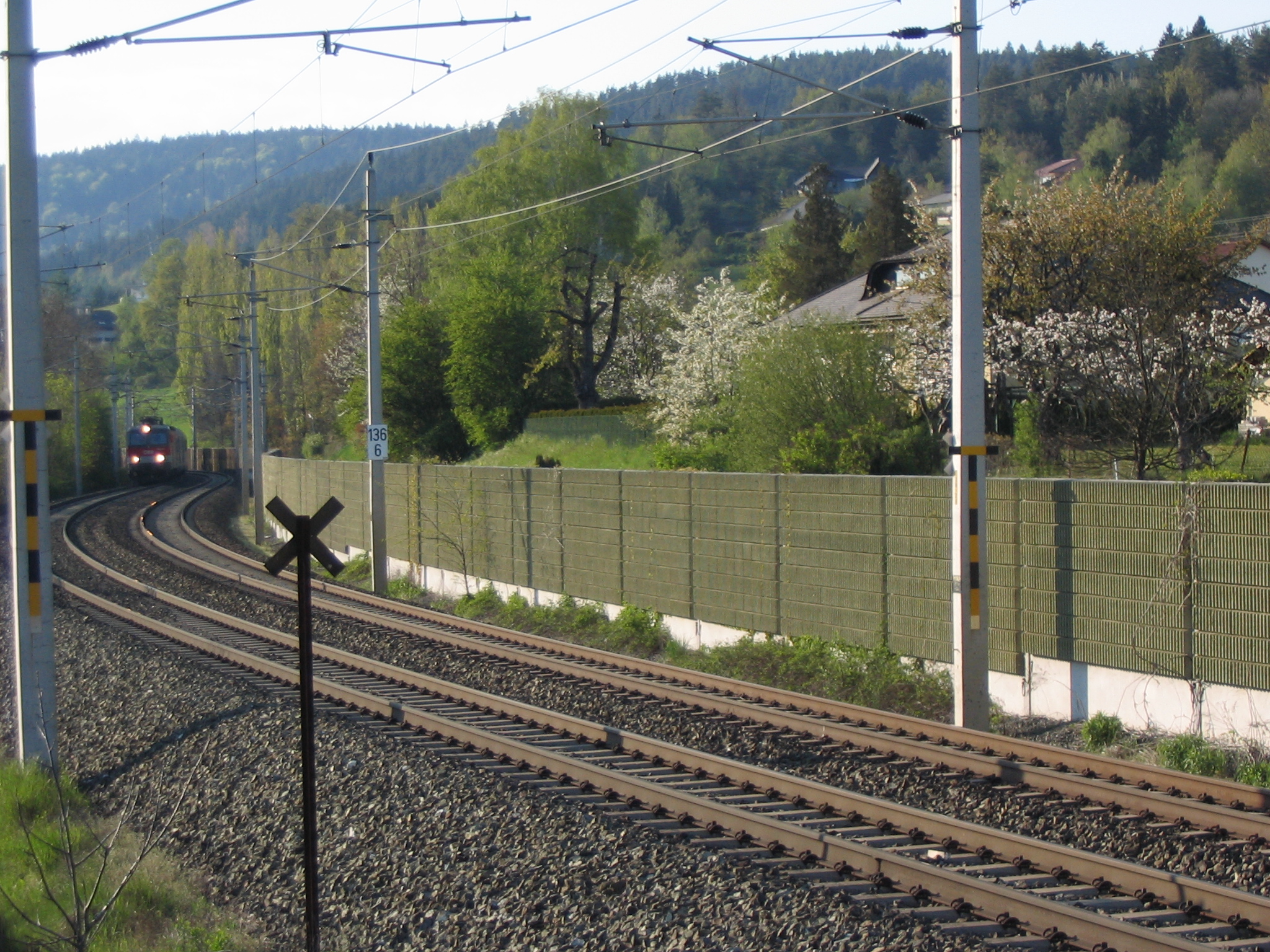
The engineering choice encompasses height, absorptive surface, maintainability, access, visual impact, snow clearance, and available corridor width. Bane NOR's technical regulations specify a minimum screen-material mass of \(15\,\mathrm{kg\,m^{-2}}\), recommend absorptive material where reflections are important, and distinguish conventional high screens from low screens placed close to the source [45]. Figure 12.15 gives one conventional trackside example: the continuous wall is placed between the railway and nearby houses, interrupting the direct line of sight from the wheel–rail source to the receivers.

Figure 12.15 Trackside noise barrier. Photo: OrdinaryHonestHardWorking, 2008, CC BY-SA 4.0 [147].

Low barriers placed close to the rail can screen low wheel–rail sources with less visual obstruction than a conventional high screen. The lecture illustrates barriers around 0.7 m high, but their effectiveness depends on source and receiver height, distance, openings and clearance requirements. They do not screen every source on the train, and neither low nor conventional airborne-noise barriers control vibration transmitted through the ground [223].

12.6.8 Protecting the Receiver

Facade, window and ventilation measures can reduce indoor airborne noise when sufficient control at the source or along the path is impractical. Their performance must be assessed with the ventilation and window conditions needed for normal occupation. They do not remove outdoor exposure and do not directly address sound arriving through the building structure.

Where ground-borne vibration or re-radiated noise governs the design, receiver measures may instead involve isolation or changes to the building’s structural response. These require a coupled assessment of the incoming vibration, foundation transmission and floor or room response. A measure should be selected for the diagnosed path rather than applying facade insulation to every noise complaint [223].

12.7 Noise in Tunnels

The acoustic environment inside a railway tunnel is fundamentally different from open air. Key phenomena include:

• Tunnel resonances: the tunnel cross-section acts as a waveguide. For an ideal rigid circular duct of radius \(r\), the first higher-order transverse mode has the cut-on frequency \(f_c \approx 1.8412c/(2\pi r)\). With \(r \approx 4.0\) m and \(c = 340\) m/s, this gives \(f_c \approx 25\) Hz; below this value, the plane mode is the only propagating acoustic mode. Real railway tunnels are not circular ducts, so modal behaviour depends on cross-section, lining, portals, and installed equipment.

• Micro-pressure waves: in high-speed tunnels a pressure wave generated by the train entrance partially converts to a micro-pressure pulse at the tunnel exit, radiating as an audible impulsive "boom" outside the tunnel portal. This is mitigated by entrance hoods and hood vents, which increase the pressure-rise time and reduce the pressure gradient before the wave reaches the tunnel exit [132, 99].

• Wheel squeal amplification: curve squeal and flange noise are amplified by the tunnel waveguide effect, particularly in curved tunnels.

Noise levels inside tunnels during train pass-by typically exceed 90–100 dB(A) at the tunnel wall, requiring careful attention to vibration in the tunnel lining and nearby structures.

12.8 Chapter Summary

Source mechanism. Rolling noise, traction noise, aerodynamic noise, impact noise, brake squeal and curve squeal are not interchangeable problems. Each source has a different dominant frequency range, speed dependence and physical origin. Rolling noise is governed mainly by combined wheel and rail roughness, while traction noise dominates at low speed and aerodynamic noise becomes important only at higher speeds. Correct diagnosis is therefore the first step in mitigation.

Transmission path. Airborne noise radiates from the wheel, rail, vehicle body or infrastructure and travels through the air to the receiver. Ground-borne vibration travels through the track, soil and building foundations, and may be felt directly or re-radiated as indoor low-frequency noise. This distinction matters because a noise barrier can reduce airborne sound but has little effect on vibration transmitted through the ground.

Assessment quantities. Railway noise is commonly described using A-weighted levels, equivalent levels and day–evening–night indices such as \(L_{den}\), while maximum levels are relevant for night-time events and sleep disturbance. Vibration assessment uses velocity-based quantities and statistical descriptors such as \(v_{w,95}\). The Norwegian regulatory framework connects these quantities to planning and assessment practice, so the engineer must understand both the physical quantity and the criterion being applied.

Mitigation chain. Rail grinding, wheel maintenance, K-block brakes and damped wheels act mainly at the source. Resilient rail pads, under-sleeper pads, under-ballast mats and floating slab track change the transmission path through the track and ground. Barriers and facade measures act closer to the receiver. A measure that is effective for one part of the chain may be ineffective or even counterproductive for another, so mitigation selection should follow the diagnosed mechanism.

Special environments. Tunnels, slab track, embedded track and dense urban corridors can change the acoustic and vibration response substantially. Tunnel waveguide effects, micro-pressure waves, re- radiated indoor noise and resilient-track deflection all require interpretation beyond a simple pass-by noise calculation. The overall implication is that railway environmental assessment extends beyond decibel arithmetic to tracing the physical path from train operation to human exposure.

Modelling and evidence. Prediction requires compatible source data, a stated propagation method and a defined receiver. Roughness spectra, track decay rate, operating state and traffic pattern explain why identical nominal train speeds can give different exposures. Lecture case studies illustrate these mechanisms; their measured reductions and planned deployments should retain their source and date.

Assignments

Assignment 1: Railway noise source diagnosis

A railway corridor passes through a residential area. Residents report four different problems:

(i) low-frequency airborne noise from a nearby station,

(ii) impulse noises from passing trains,

(iii) a tonal "singing" noise on the nearby track, and

(iv) a sharp squeal from a nearby station.

(a) Identify the likely source of each complaint. Consider traction or auxiliary noise, rolling noise, corrugation, brake or curve squeal, impact noise, aerodynamic noise and ground-borne vibration. Where the description permits more than one explanation, state what additional observation is needed.

(b) For each complaint, identify whether the first investigation should focus mainly on the vehicle, the wheel–rail contact, the track condition, the propagation path, or the receiver.

(c) Choose one measurement or inspection method that would help confirm each diagnosis.

Assignment 2: Rolling noise speed and roughness

A freight train travels at \(v_1 = 100\) km/h and generates a pass-by noise level of \(L_A = 82\) dB(A) at 25 m from the track.

(a) Using \(\Delta L_A = 30\log_{10}(v_2/v_1)\), calculate the rolling-noise level if speed is increased to \(v_2 = 160\) km/h.

(b) For the original train at 100 km/h, assume the wheel roughness level in the dominant wavelength band is \(L_{r,w}=46\) dB and the rail roughness level is \(L_{r,r}=42\) dB. After an approved conversion from cast-iron blocks to K-blocks with the necessary braking-system adaptations, the wheel roughness falls to \(L_{r,w}=36\) dB while the rail roughness is unchanged. Use

\[ L_{r,\mathrm{comb}} = 10\log_{10}\!\left(10^{L_{r,w}/10}+10^{L_{r,r}/10}\right) \]

to estimate the change in combined roughness and the corresponding rolling-noise reduction.

(c) Explain why this rolling-noise reduction is smaller than the 10 dB reduction in wheel roughness.

(d) State why aerodynamic noise is not normally the controlling source for this freight-train speed range.

Assignment 3: Day–evening–night railway noise assessment

A dwelling located 30 m from a railway line experiences the following equivalent noise levels: \(L_d = 62\) dB(A) (daytime), \(L_e = 58\) dB(A) (evening), \(L_n = 55\) dB(A) (night).

(a) Calculate \(L_{den}\) for the dwelling and comment on whether it satisfies the relevant T-1442 railway planning value.

(b) Explain why this differs from the T-1442 nighttime maximum-level check using \(L_{5AF}\).

(c) If source and path measures reduce all three equivalent levels by 8 dB(A), recalculate \(L_{den}\) and comment on compliance.

(d) State the assessment context and the assumptions needed for a compliance conclusion.

Assignment 4: Mitigation choice for noise and vibration

A mixed passenger and freight line runs close to housing and then enters a short tunnel below a vibration-sensitive building. Measurements show outdoor rolling noise and indoor low-frequency rumble. A resilient-track option changes the simplified track support stiffness from \(C_t = 120\) to 60 kN/mm. Use \(Q = 100\) kN.

(a) Propose one source measure, one propagation-path measure, and one receiver measure. State which problem each measure addresses.

(b) Using \(\delta = Q/C_t\), compare rail deflection before and after the resilient-track option. Why is this only an indicator?

(c) Explain how under-sleeper pads or softer rail support can reduce vibration transmission, and state one disadvantage.

(d) Is a conventional noise barrier alone sufficient? Justify the answer using the source–path–receiver framework.